THE AUDITORY MODELING TOOLBOX
This documentation page applies to an outdated major AMT version. We show it for archival purposes only.
Click here for the documentation menu and here to download the latest AMT (1.6.0).
EXP_GAMMATONE - Creates various figures related to the Gammatone filters
Usage
exp_gammatone(flags)
exp_gammatone(flags) reproduces some figures from Patterson et al. (1987), Lyon (1997), and Hohmann (2002)
The following flags can be specified;
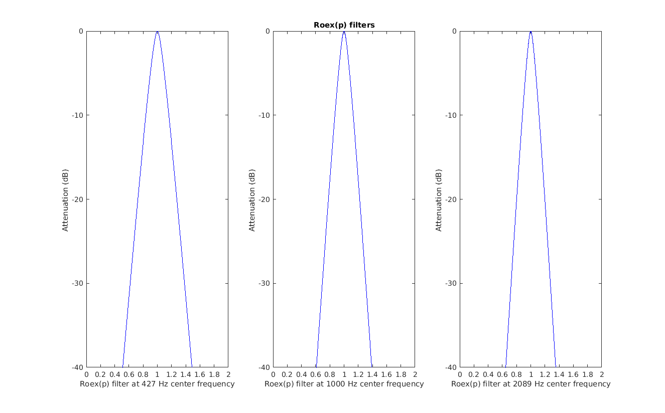
'fig1_patterson1987''
Reproduce Fig.1 from Patterson et al. (1987): The amplitude characteristics of three roex(p) filters centered at 427 Hz, 1000 Hz and 2089 Hz. The lower and upper filters are centered 6 ERBs below and above the 1000 Hz filter respectively. In each case, the range of the abscissa extends from an octave below to an octave above the centre frequency of the filter, on a linear frequency scale. The range of the ordinate is 40dB.
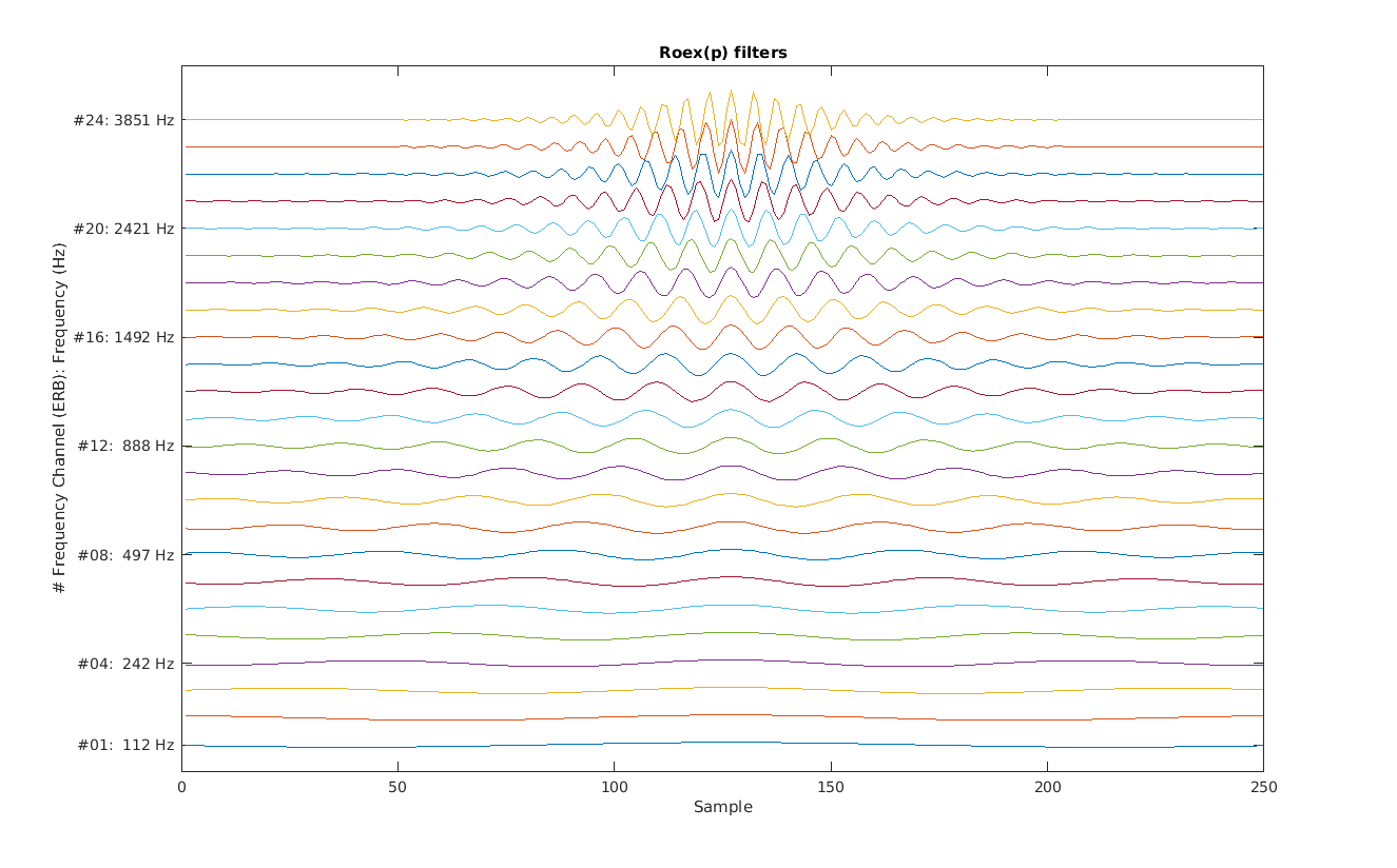
'fig2_patterson1987''
Reproduce Fig.2 from Patterson et al. (1987): An array of 24 impulse responses for roex(p) filters whose centre frequencies ranges from 100 to 4000 Hz. The linear-phase assumption leads to symmetric impulse responses which have been aligned at their temporal mid-points.
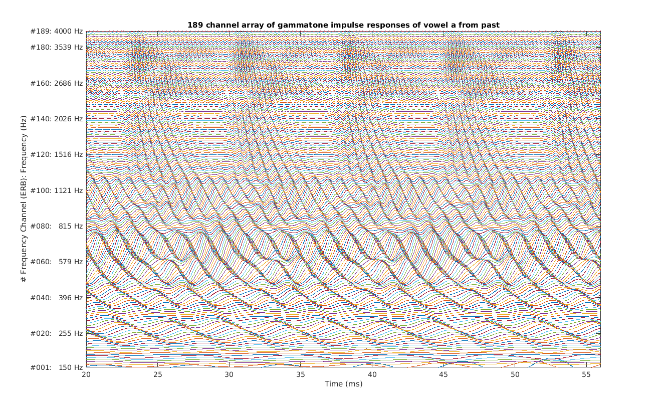
'fig3_patterson1987''
Reproduce Fig.3 similiar to Patterson et al. (1987): A cochleagram of four cycles of the [ae] in "past" produced by by a gammatone filterbank without phase compensation. The triangular objects are the upper three formants of the vowel. The duration of each period is ~8 ms. The ordinate is filter centre frequency of 189 equally spaced channels from 100 to 4000 Hz. Note the strong rightward skew induced by the phase lags of the low-frequency filters in the lower half of the figure.
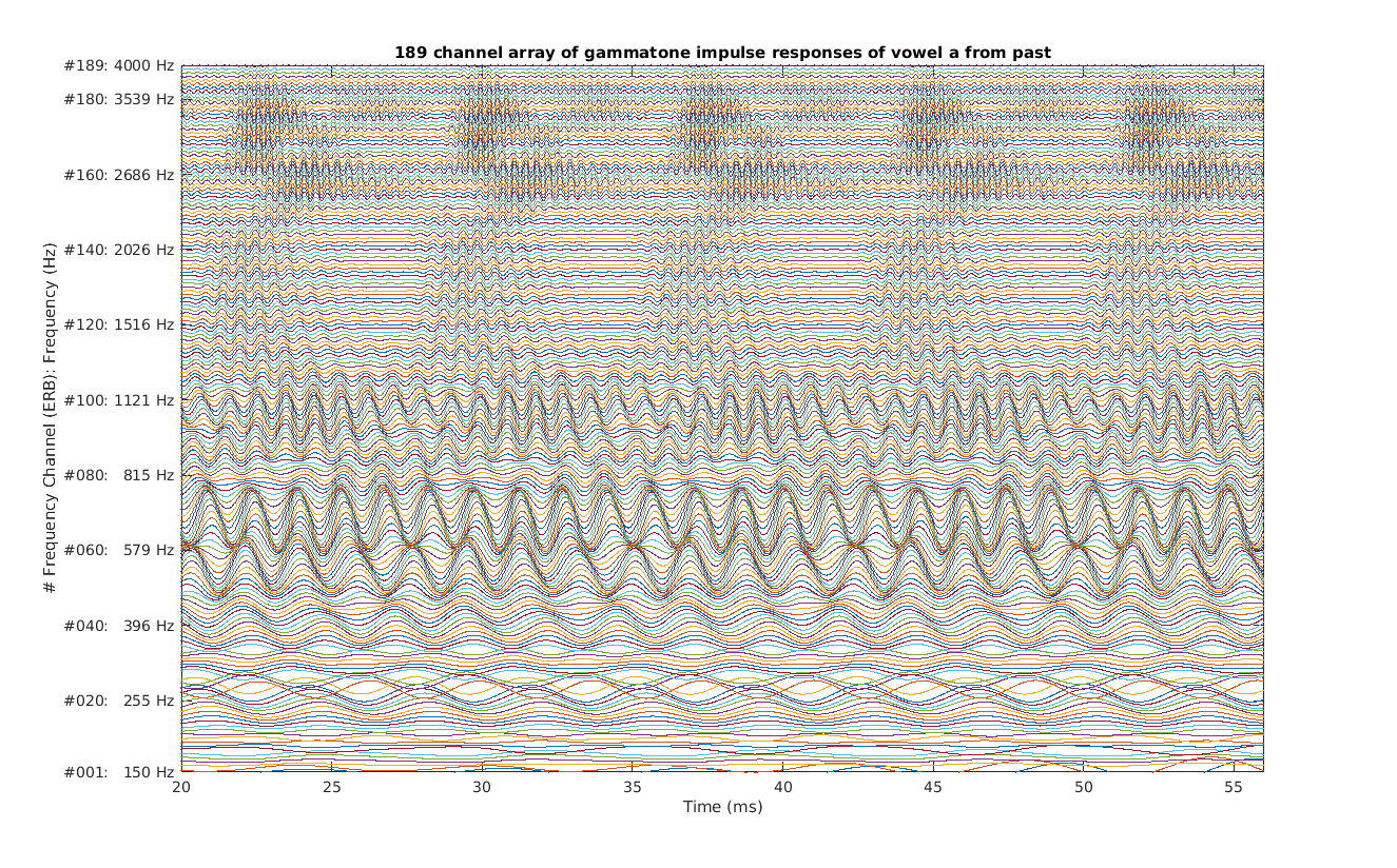
'fig4_patterson1987''
Reproduce Fig.4 similiar to Patterson et al. (1987): A cochleagram of four cycles of the [ae] in "past" produced by a gammatone filterbank with phase compensation. The coordinates are the same as for Figure 3. Note that the strong rightward skew produced by the phase lags of the lower frequency filters has been removed now.
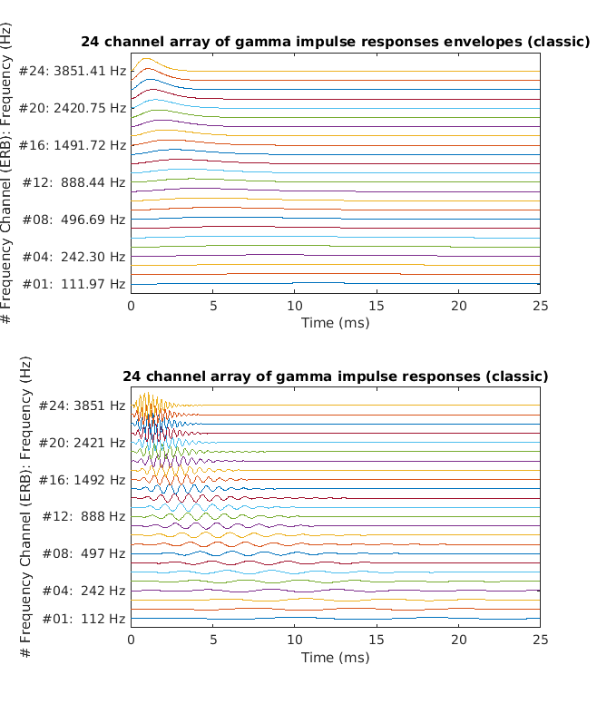
'fig5_patterson1987''
Reproduce Fig.5 from Patterson et al. (1987): An array of gamma impulse responses for a 24-channel auditory filterbank.(lower portion), and the equvalent array of gamma envelopes (upper portion). The range of abcissa is 25 ms; the filter centre frequencies range from 100 - 4,000 Hz.
'fig6_patterson1987''
Reproduce Fig.6 from Patterson et al. (1987): A comparison of the gammatone(4,b) and roex(p) filters at three centre frequencies, 0.43, 1.00 and 2.09 kHz. In this case, the gammatone filter has been matched to the roex filter by equating the ERB, thus minimising the difference in the area under the curves. The range of the ordinate is 60 dB, the abscissa ranges from an octave below to an octave above the centre frequency in each case.
'fig7_patterson1987''
Reproduce Fig.7 from Patterson et al. (1987): The comparison of the gammatone(4,b) and roex(p) filters at three centre frequencies (0.43, 1.00 and 2.09 kHz). In this case, the bandwidth of the gammatone filter has been increased by 10% to minimise the decibel difference between it and the roex filter. The range of the ordinate is 60 dB, and the abscissa ranges from an octave below to an octave above the centre frequency of the filter in each case.
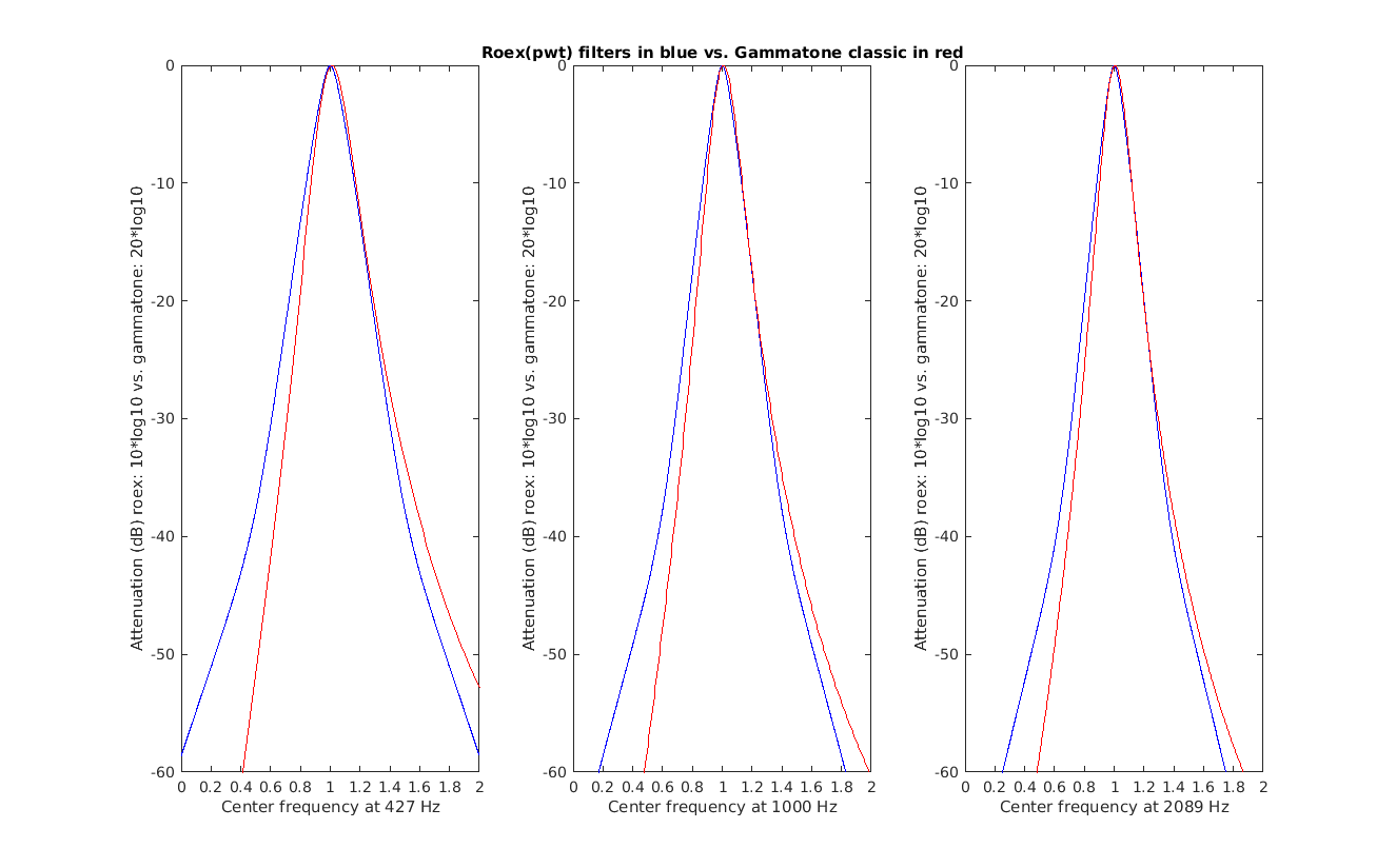
'fig8_patterson1987''
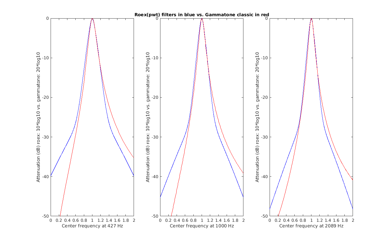
Reproduce Fig.8 from Patterson et al. (1987): A comparison of the gammatone(2,b) and the roex(p,w,t) filters at three centre frequencies (0.43, 1.00 and 2.09 kHz). The parameters for the roex filter are taken from Patterson et al (1982). The gammatone filter has been fitted to the roex by equating their ERBs. The range of the ordinate is 50dB, and the abscissa ranges from an octave below to an octave above the centren frequency, in each case.
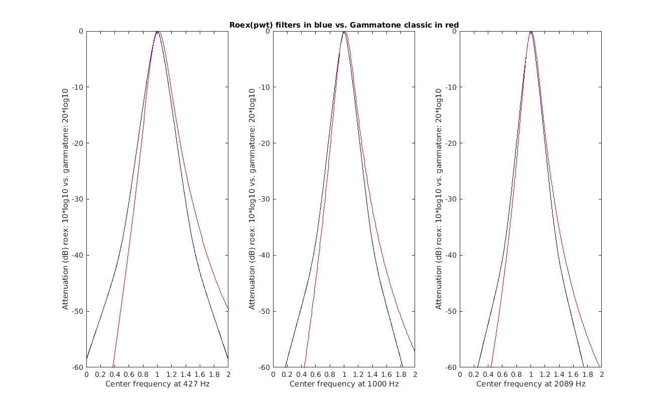
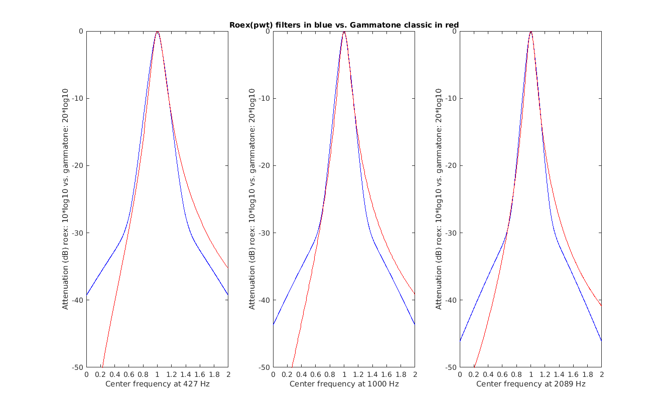
'fig9_patterson1987''
Reproduce Fig.9 from Patterson et al. (1987): A comparison of the gammatone(2,b) and the roex(p,w,t) filters at three centre frequencies (0.43, 1.00 and 2.09 kHz). In this case the roex parameters, w and t, have been adjusted to improve the fit to the gammatone(2,b) filter to show that the discrepancy can easily be minimised. The range of the ordinate is 50 dB, the abscissa shows a range from an octave below to an octave above the centre frequency of the filter in each case.
'fig10a_patterson1987''
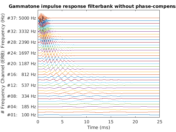
Reproduce Fig.10a from Patterson et al. (1987): The impulse responses for a gammatone auditory filterbank without phase compensation. The filterbank contains 37 channels ranging from 100 to 5,000 Hz. The range of abcissa is 25 ms.
'fig10b_patterson1987''
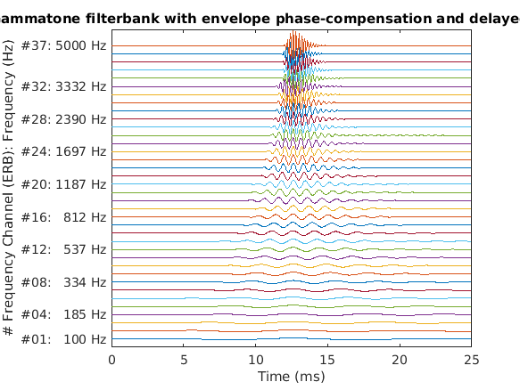
Reproduce Fig.10b from Patterson et al. (1987): The impulse responses for a gammatone auditory filterbank with envelope phase-compensation; that is, the peaks of the impulse-response envelopes have been aligned vertically. The filterbank contains 37 channels ranging from 100 to 5,000 Hz. The range of the abscissa is 25 ms.
'fig10c_patterson1987''
Reproduce Fig.10c from Patterson et al. (1987): The impulse responses for a gammatone auditory filterbank with envelope and fine structure phase-compensation; that is, the envelope peaks have been aligned and then a fine structure peak has been aligned with the envelope peak. The filterbank contains 37 channels ranging from 100 to 5,000 Hz. The range of abcissa is 25 ms.
'fig11_patterson1987''
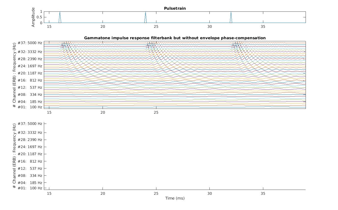
Reproduce similiar to Fig.11 from Patterson et al. (1987): The impulse responses of a gammatone filterbank from a pulsetrain.
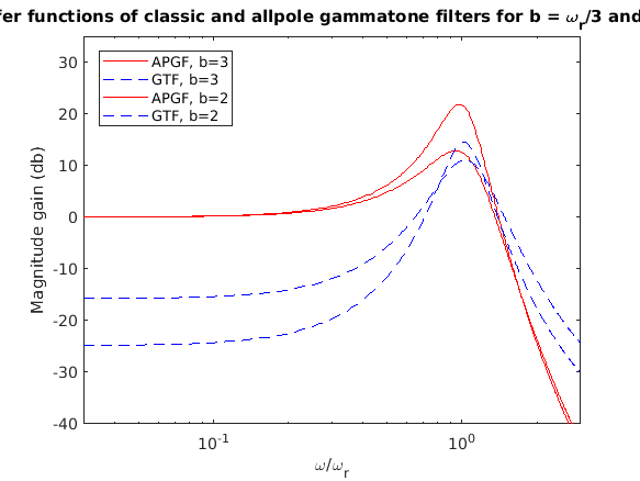
'fig1_lyon1997''
Reproduce parts of Fig.1 from Lyon (1997) (no DAPGF): Comparison of GTF and APGF transfer function for two different values of the real part of the pole position. Notice that the ordering of gain near the peak for the classic gammatone filter is not maintained in the tail. The variation in the GTF tail is not accounted for by the usual phase-independent symetric GTF approximation.
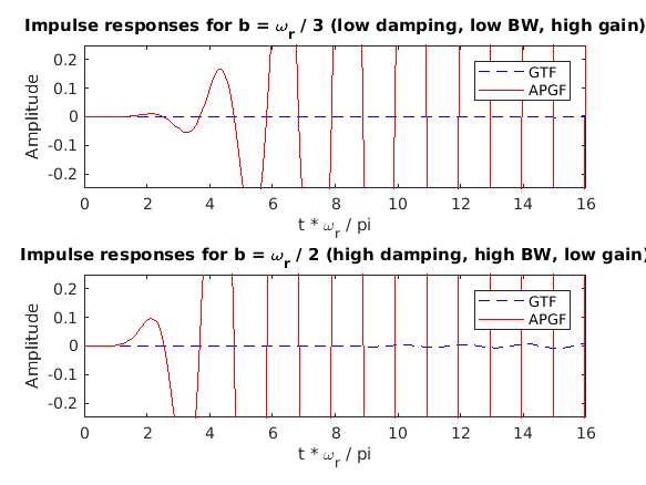
'fig2_lyon1997''
Reproduce parts of Fig.2 from Lyon (1997) (no DAPGF): Impulse responses of the APGF and sine-phased GTF from Figure 1. Note that the GTF's zero crossings are equally spaced in time, while those of the APGF are stretched out in early cycles.
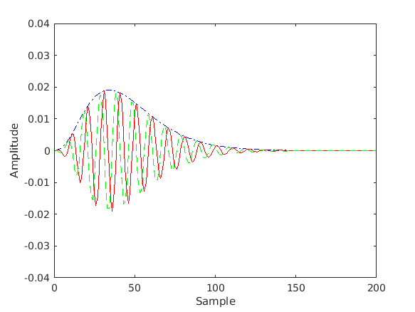
'fig1_hohmann2002''
Reproduce Fig.l from Hohmann (2002): Impulse response of the example Gammatone filter (center frequency fc = 1000 Hz; 3-db bandwidth fb = 100 Hz; sampling frequency fs = 10kHz). Solid and dashed lines show the real and imaginary part of the filter output, respectively. The absolute value of the filter output (dashdotted line) clearly represents the envelope.
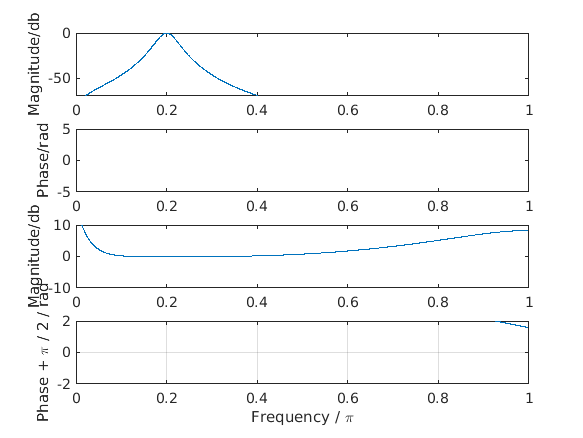
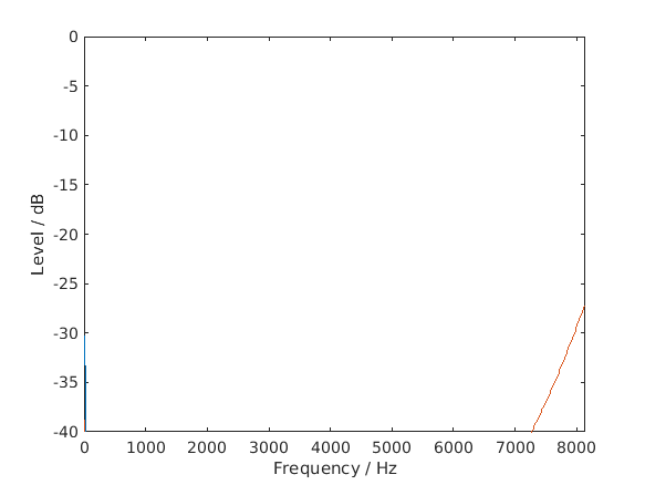
'fig2_hohmann2002''
Reproduce Fig.2 from Hohmann (2002): Frequency response of the example Gammatone filter (upper two panels) and of the real-to-imaginary response(lower two panels). Pi/2 was added to the phase of the latter (see text). The frequency axis goes up to half the sampling rate (z=pi).
'fig3_hohmann2002''
Reproduce Fig.3 from Hohmann (2002): Magnitude frequency response of the Gammatone filterbank. In this example, the filter channel density is 1 on the ERB scale and the filter bandwidth is 1 ERBaud. The sampling frequency was 16276Hz and the lower and upper boundary for the center frequencies were 70Hz and 6.7kHz, respectively.
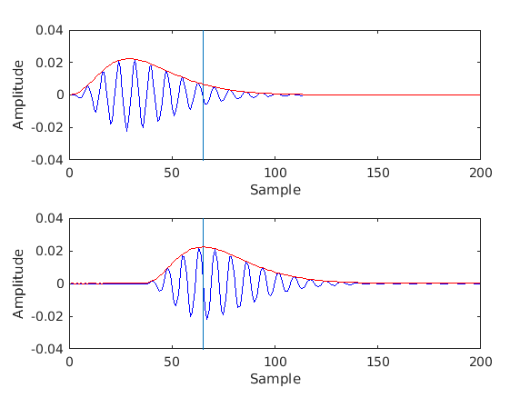
'fig4_hohmann2002''
Treatment of an impulse response with envelope maximum to the left of the desired group delay (at sample 65). The original complex impulse response (real part and envelope plotted in the upper panel) is multiplied with a complex factor and delayed so that the envelope maximum and the maximum of the real part coincide with the desired group delay (lower panel).
Examples:
To display Fig. 1 from Patterson et al. (1987) use
exp_gammatone('fig1_patterson1987');
To display Fig. 2 Patterson et al. (1987) use
exp_gammatone('fig2_patterson1987');
To display Fig. 3 Patterson et al. (1987) use
exp_gammatone('fig3_patterson1987');
To display Fig. 4 Patterson et al. (1987) use
exp_gammatone('fig4_patterson1987');
To display Fig. 5 Patterson et al. (1987) use
exp_gammatone('fig5_patterson1987');
To display Fig. 6 Patterson et al. (1987) use
exp_gammatone('fig6_patterson1987');
To display Fig. 7 Patterson et al. (1987) use
exp_gammatone('fig7_patterson1987');
To display Fig. 8 Patterson et al. (1987) use
exp_gammatone('fig8_patterson1987');
To display Fig. 9 Patterson et al. (1987) use
exp_gammatone('fig9_patterson1987');
To display Fig. 10a Patterson et al. (1987) at use
exp_gammatone('fig10a_patterson1987');
To display Fig. 10b Patterson et al. (1987) at use
exp_gammatone('fig10a_patterson1987');

To display Fig. 10c Patterson et al. (1987) at use
exp_gammatone('fig10c_patterson1987');
To display Fig. 11 Patterson et al. (1987) use
exp_gammatone('fig11_patterson1987');
To display Fig. 1 Lyon (1997) use
exp_gammatone('fig1_lyon1997');
To display Fig. 2 Lyon (1997) use
exp_gammatone('fig2_lyon1997');
To display Fig. 1 Hohmann (2002) use
exp_gammatone('fig1_hohmann2002');
To display Fig. 2 Hohmann (2002) use
exp_gammatone('fig2_hohmann2002');
To display Fig. 3 Hohmann (2002) use
exp_gammatone('fig3_hohmann2002');
To display Fig. 4 Hohmann (2002) use
exp_gammatone('fig4_hohmann2002');
References:
V. Hohmann. Frequency analysis and synthesis using a gammatone filterbank. Acta Acustica united with Acoustica, 88(3):433--442, 2002.
R. Lyon. All pole models of auditory filtering. In E. R. Lewis, G. R. Long, R. F. Lyon, P. M. Narins, C. R. Steele, and E. Hecht-Poinar, editors, Diversity in auditory mechanics, pages 205--211. World Scientific Publishing, Singapore, 1997.
B. Moore and B. Glasberg. Suggested formulae for calculating auditory-filter bandwidths and excitation patterns. J. Acoust. Soc. Am., 74:750--753, 1983.
R. Patterson, I. Nimmo-Smith, J. Holdsworth, and P. Rice. An efficient auditory filterbank based on the gammatone function. APU report, 2341, 1987.


Build with Bootstrap