THE AUDITORY MODELING TOOLBOX
This documentation page applies to an outdated major AMT version. We show it for archival purposes only.
Click here for the documentation menu and here to download the latest AMT (1.6.0).
EXP_ZIEGELWANGER2013 - Figures from Ziegelwanger and Majdak (2013)
Usage
data = exp_ziegelwanger2013(flag)
Description
exp_ziegelwanger2013(flags) reproduces figures of the paper from Ziegelwanger and Majdak (2013).
Optional fields of output data structure:
The following flags can be specified:
| 'plot' | Plot the output of the experiment. This is the default. |
| 'noplot' | Don't plot, print results in the console. |
'reload' Reload previously calculated results. This is the default.'
'recalc' Recalculate results.'
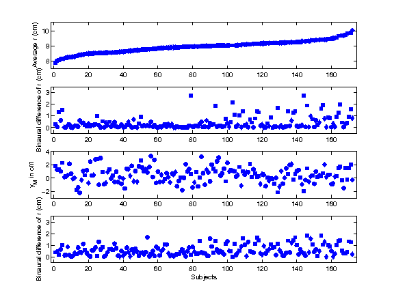
| 'fig1a' | Reproduce Fig. 1 from ziegelwanger2013: Model parameters (sphere radius, sphere center) resulting from fitting the off-axis model to HRTFs of human listeners. |
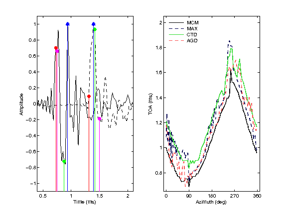
| 'fig1b' | Reproduce Fig. 1 from majdak2013: Left panel: Normalized HRIRs of NH89 (ARI database). Sound source was placed 45 deg left in the horizontal plane. Solid line: for the left ear Dashed line: for the right ear Vertical lines: Estimated TOAs Arrows: Resulting ITDs from the corresponding TOAs Circles, Red: Minimum-Phase Cross-Correlation Method Triangle, Green: Time-Position of the HRIR-Maximum Diamonds, Blue: Centroid of the HRIR Squares, Magenta: Average Group Delay (1-5 kHz) Right panel: Estimated TOAs of NH89 (ARI database) in the horizontal interaural plane. Black: Minimum-Phase Cross-Correlation Method Blue: Time-Position of the HRIR-Maximum Green: Centroid of the HRIR Red: Average Group Delay (1-5 kHz) |
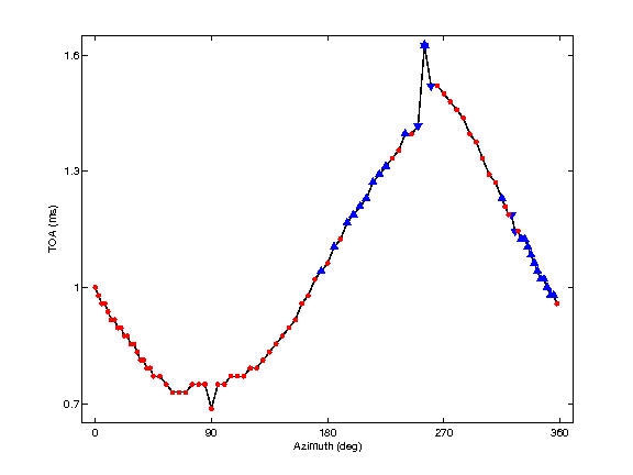
| 'fig2b' | Reproduce Fig. 2 from majdak2013: Right panel: Estimated TOAs, detected outliers and outlier adjusted set of TOAs for NH89 (ARI database) in the horizontal plane. Line: Estimated TOAs Triangles (down), Blue: Detected outliers for the azimuthal slope criterion Triangles (up), Blue: Detected outliers for the sagittal variance criterion Dots, Red: Outlier-adjusted set |
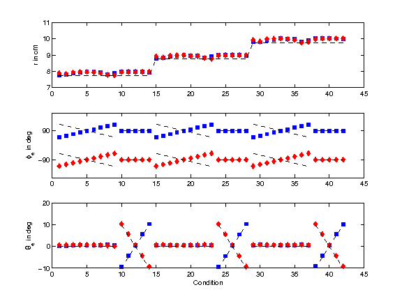
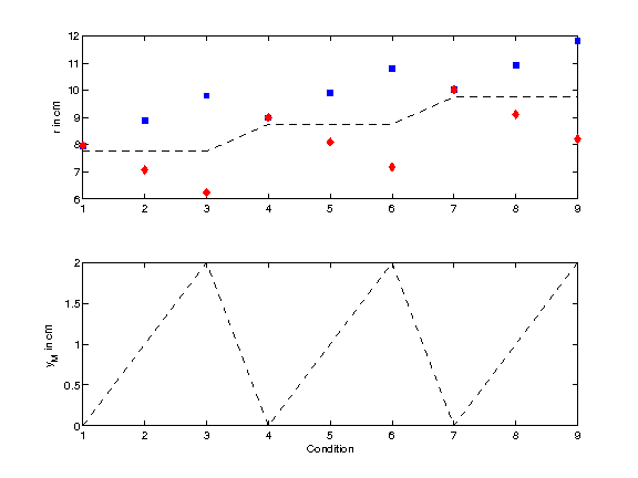
| 'fig3b' | Reproduce Fig. 3 from majdak2013: Left panel: Model parameters (sphere radius, ear position) resulting from fitting the on-axis model to HRTFs of a rigid sphere. Squares: for the left ear Diamonds: for the right ear Dashed lines: set values used in the numerical HRTF calculation Right panel: Model parameters (sphere radius) resulting from fitting the on-axis model to HRTFs of an off-axis placed rigid sphere. |
Examples:
To display Fig. 1a, use
exp_ziegelwanger2013('fig1a');
To display Fig. 1b, use
exp_ziegelwanger2013('fig1b');
This code produces the following output:
MAX: ITD is 0.4375 ms
CTD: ITD is 0.52083 ms
AGD: ITD is 0.72917 ms
MCM: ITD is 0.5625 ms
To display Fig. 2b, use
exp_ziegelwanger2013('fig2b');
To display Fig. 3b, use
exp_ziegelwanger2013('fig3b');
References:
P. Majdak and H. Ziegelwanger. Continuous-direction model of the broadband time-of-arrival in the head-related transfer functions. In ICA 2013 Montreal, volume 19, page 050016, Montreal, Canada, 2013. ASA. [ DOI ]
H. Ziegelwanger and P. Majdak. Modeling the broadband time-of-arrival of the head-related transfer functions for binaural audio. In Proceedings of the 134th Convention of the Audio Engineering Society, page 7, Rome, 2013.


Build with Bootstrap