THE AUDITORY MODELING TOOLBOX
This documentation page applies to an outdated major AMT version. We show it for archival purposes only.
Click here for the documentation menu and here to download the latest AMT (1.6.0).
EXP_BAUMGARTNER2014 - Figures from Baumgartner et al. (2014)
Usage
data = exp_baumgartner2014(flag)
Description
exp_baumgartner2014(flag) reproduces figures of the study from Baumgartner et al. (2014).
Optional fields of output data structure:
- data.contralateralGain
- contralateral gain of binaural weighting function
The following flags can be specified;
| 'plot' | Plot the output of the experiment. This is the default. |
| 'noplot' | Don't plot, only return data. |
| 'autorefresh' | Re-calculate the file if it does not exist. Return 1 if the file exist, otherwise 0. This is the default |
| 'refresh' | Always recalculate the file. |
| 'cached' | Always use the cached version. Throws an error if the file does not exist. |
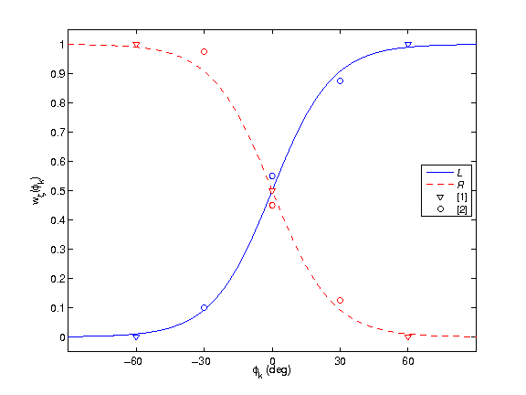
| 'fig2' | Reproduce Fig.2: Binaural weighting function best fitting results from Morimoto (2001) labeled as [1] and Macpherson and Sabin (2007) labeled as [2] in a squared error sense. |
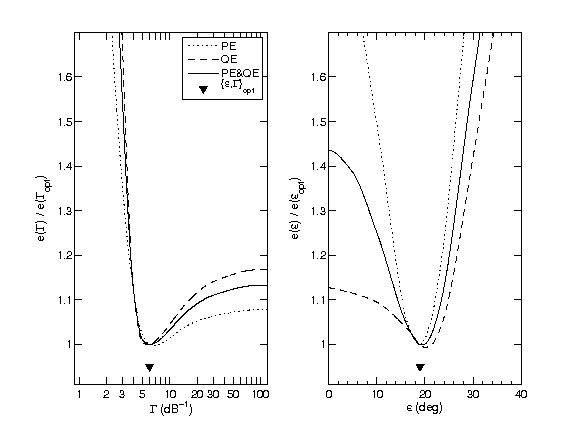
| 'fig3' | Reproduce Fig.3: Partial and joint prediction residues, \(e_\mathrm{PE}\) and/or \(e_\mathrm{QE}\) , as functions of the degree of selectivity, \(\Gamma\) , and the motoric response scatter, \(\varepsilon\) . Residuum functions are normalized to the minimum residuum obtained for the optimal parameter value. See text for details. |
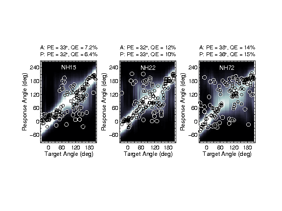
| 'fig4' | Reproduce Fig.4: Actual and predicted response patterns of listeners NH15, NH22, and NH72 (from left to right) when listening to targets in the baseline condition and in the midsagittal plane. Actual response angles are shown as open circles. Probabilistic response predictions are encoded by brightness according to the color bar to the right. Actual (A) and predicted (P) performances (PEs and QEs) of the listener are listed above each panel. |
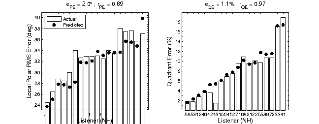
| 'fig5' | Reproduce Fig.5: Listener-specific baseline performance in the midsagittal plane. Local performance is shown in terms of PE (left), global performance in terms of QE (right). Correlation coefficients, \(r\) , and prediction residues, \(e\) , with respect to actual and predicted performances are shown above each panel. |
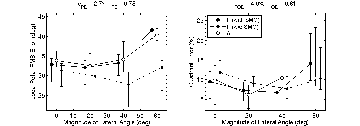
| 'fig6' | Reproduce Fig.6: Baseline performance as a function of the magnitudes of the lateral response angle. Symbols and whiskers show median values and inter-quartile ranges, respectively. Symbols were horizontally shifted to avoid overlaps. Correlation coefficients, \(r\) , and prediction residues, \(e\) , specify the correspondence between actual (A) and predicted (P) listener-specific performances. Predictions of the model without the sensory-motoric mapping (SMM) stage are shown with dashed lines. |
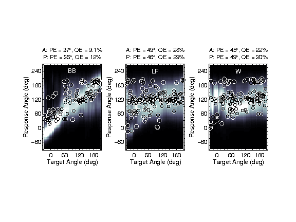
| 'fig7' | Reproduce Fig.7: Actual and predicted response patterns of listener NH62 when listening to broadband (left), low-pass filtered (center), or spectrally warped (right) DTFs of the midsagittal plane. Data were pooled within \(\pm15^\circ\) of lateral angle. All other conventions are as in Fig.4. |
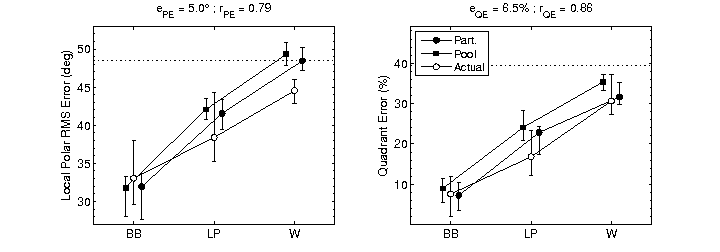
| 'fig8' | Reproduce Fig.8: Effect of band limitation and spectral warping. Listeners were tested with broadband (BB), low-pass filtered (LP), and spectrally warped (W) DTFs. Actual: experimental results from Majdak et al. (2013). Part.: Model predictions for the actual eight participants based on the actually tested target positions. Pool: Model predictions for our pool of 18 listeners based on all possible target positions. Dotted horizontal lines represent chance rate. All other conventions are as in Fig.6. |
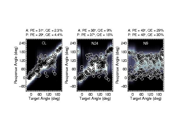
| 'fig9' | Reproduce Fig.9: Actual and predicted response patterns of exemplary listener NH12 listening to channel-limited HRTFs. Results for an unlimited number of channels (broadband click trains), 24, and 9 channels are shown from left to right. All other conventions are as in Fig.7. |
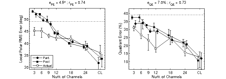
| 'fig10' | Reproduce Fig.10: Effect of spectral resolution in terms of varying the number of spectral channels used by a channel vocoder. Actual experimental results are from Goupell et al. (2010). Stimulation with broadband click trains (CL) represents an unlimited number of channels. All other conventions are as in Fig.8. |
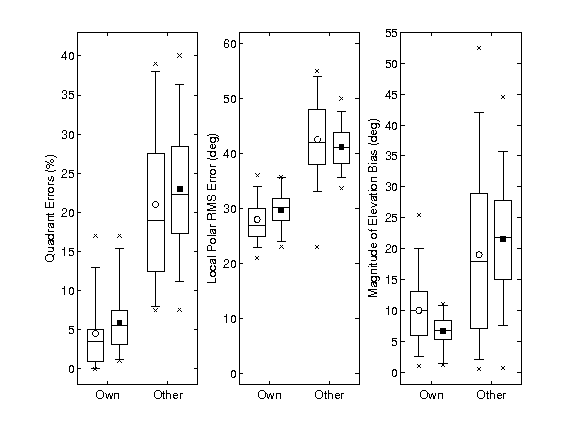
| 'fig11' | Reproduce Fig.11: Effect of non-individualized HRTFs, i.e., localizing with others' instead of own ears. Statistics summary replotted from Fig.13 of Middlebrooks (1999b). Horizontal lines represent 25th, 50th, and 75th percentiles, the whiskers represent 5th and 95th percentiles, and crosses represent minima and maxima. Circles and squares represent mean values. |
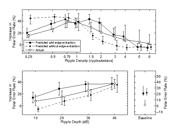
| 'fig12' | Reproduce Fig.12: Effect of spectral ripples. Actual experimental results are from Macpherson et al. (2003). Either the ripple depth of 40dB (top) or the ripple density of one ripple/octave (bottom) was kept constant. Predictions (P) of the model without the DCN stage are shown with dashed lines. All other conventions are as in Fig.8. |
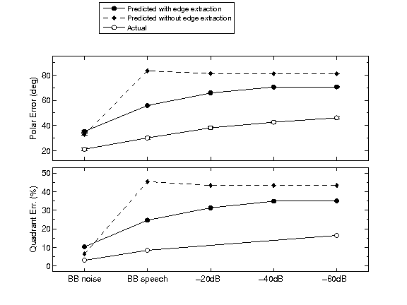
| 'fig13' | Reproduce Fig.13: Effect of high-frequency attenuation in speech. Actual experimental results are from Best et al. (2005). Open and filled symbols show actual and predicted results, respectively. Absolute polar angle errors (top) and QEs (bottom) averaged across listeners are shown. |
Requirements:
- SOFA API from http://sourceforge.net/projects/sofacoustics for Matlab (in e.g. thirdparty/SOFA)
- Data in hrtf/baumgartner2014
- Statistics Toolbox for Matlab (for some of the figures)
Examples:
To display Fig.2 use
exp_baumgartner2014('fig2');
This code produces the following output:
Phi: 13 deg
To display Fig.3 use
exp_baumgartner2014('fig3');
To display Fig.4 use
exp_baumgartner2014('fig4');
To display Fig.5 use
exp_baumgartner2014('fig5');
To display Fig.6 use
exp_baumgartner2014('fig6');
To display Fig.7 use
exp_baumgartner2014('fig7');
This code produces the following output:
Listener: NH39
To display Fig.8 use
exp_baumgartner2014('fig8');
To display Fig.9 use
exp_baumgartner2014('fig9');
This code produces the following output:
Listener: NH12
To display Fig.10 use
exp_baumgartner2014('fig10');
To display Fig.11 use
exp_baumgartner2014('fig11');
To display Fig.12 use
exp_baumgartner2014('fig12');
This code produces the following output:
Correlation between actual and predicted median values (15 conditions):
w/  DCN: r = 0.89
w/o DCN: r = 0.78
To display Fig.13 use
exp_baumgartner2014('fig13');
References morimoto2001 macpherson2007


Build with Bootstrap