THE AUDITORY MODELING TOOLBOX
This documentation page applies to an outdated major AMT version. We show it for archival purposes only.
Click here for the documentation menu and here to download the latest AMT (1.6.0).
LINDEMANN1986 - Calculates a binaural activation pattern
Usage
[crosscorr,t] = lindemann1986(insig,fs,c_s,w_f,M_f,T_int,N_1)
[crosscorr,t] = lindemann1986(insig,fs,c_s,w_f,M_f,T_int)
[crosscorr,t] = lindemann1986(insig,fs,c_s,w_f,M_f)
[crosscorr,t] = lindemann1986(insig,fs,c_s,w_f)
[crosscorr,t] = lindemann1986(insig,fs,c_s)
[crosscorr,t] = lindemann1986(insig,fs)
Input parameters
| insig | binaural signal for which the cross-correlation should be calculated |
| fs | sampling rate (Hz) |
Output parameters
| crosscorr | A matrix containing the cross-correlation signal for every frequency channel fc and every time step n. The format of this matrix is output(n,m,fc), where m denotes the correlation (delay line) time step. |
| t | time axis for the time steps n in crosscorr |
| ild | interaural level difference (ILD) for every freqeuncy channel fc |
| cfreq | center frequencies of every frequency channel |
Description
lindemann1986(insig,fs) calculates a binaural activity map for the given insig using a cross-correlation (delay-line) mechanism. The calculation is done for every frequency band in the range 5-40 Erb.
Lindemann has extended the delay line model of Jeffres (1948) by a contralateral inhibition, which introduce the ILD to the model. Also monaural detectors were extended, to handle monaural signals (and some stimuli with a split off of the lateralization image). Hess has extented the output from the Lindemann model to a binaural activity map dependend on time, by using a running cross-correlation function. This has been done here by starting a new running cross-correlation every time step T_int. A detailed description of these cross- correlation steps is given in the lindemann1986bincorr function.
The steps of the binaural model to calculate the result are the following:
- The given stimulus is filtered using an erb bank to get 36 frequency bands containing a stimulus waveform.
- In a second step the auditory nerve is siumulated by extracting the envelope using a first order low pass filter with a cutoff frequency of 800 Hz and half-wave rectification.
- Calculation of the cross-correlation between the left and right channel. This is done using the model described in Lindemann (1986a) and Hess (2007). These are extensions to the delay line model of Jeffres (1948).
You may supply any flags or key/value pairs of the auditoryfilterbank, ihcenvelope or lindemann1986bincorr at the end of the line of input arguments.
Examples:
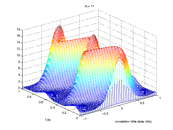
This example shows how to the binaural activity map for one frequency channel of the Lindemann binaural model for a sinusoid with a binaural modulation rate of 2 Hz.
fs = 44100; % Sampling rate
f = 500;    % Frequency of the sinusoid
mf = 2;     % Binaural modulation frequency

% Generate 1~s binaural modulated sinusoid
sig = bmsin(f,mf,fs);

% Model paramter (Note: T_int (ms) should be a multiple of 1000/f == 2)
% Begin of the storage of the cross-correlation is set to 1, because we have a
% non-stationary signal

% Calculate binaural cross-correlation
[cc,t] = lindemann1986(sig,fs,'T_int',6);

% Plot frequency channel 11, due to round(freqtoerb(500))==11
plot_lindemann1986(cc,t,'fc',f);
References:
W. Gaik. Combined evaluation of interaural time and intensity differences: Psychoacoustic results and computer modeling. J. Acoust. Soc. Am., 94:98-110, 1993.
W. Hess. Time-Variant Binaural-Activity Characteristics as Indicator of Auditory Spatial Attributes. PhD thesis, Ruhr-Universitaet Bochum, 2007.
L. Jeffress. A place theory of sound localization. Journal of comparative and physiological psychology, 41(1):35-39, 1948.
W. Lindemann. Extension of a binaural cross-correlation model by contralateral inhibition. I. Simulation of lateralization for stationary signals. J. Acoust. Soc. Am., 80:1608-1622, 1986.
W. Lindemann. Extension of a binaural cross-correlation model by contralateral inhibition. II. The law of the first wave front. J. Acoust. Soc. Am., 80:1623-1630, 1986.


Build with Bootstrap