THE AUDITORY MODELING TOOLBOX
This documentation page applies to an outdated major AMT version. We show it for archival purposes only.
Click here for the documentation menu and here to download the latest AMT (1.6.0).
EXP_ZIEGELWANGER2014 - Figures from Ziegelwanger and Majdak (2014)
Usage
data = exp_ziegelwanger2014(flag)
Description
exp_ziegelwanger2014(flags) reproduces figures of the paper from Ziegelwanger and Majdak (2014).
The following flags can be specified:
| 'redo' | Recalculate results. |
| 'cached' | Use cached results. Default. |
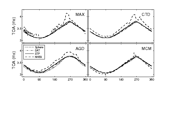
| 'fig3' | Reproduce Fig. 3: TOAs resulting from TOA estimators in the horizontal plane applied on calculated HRTFs of the objects Sphere, SAT, STP, as well on measured HRTFs of an exemplary listener (NH89, ARI). |
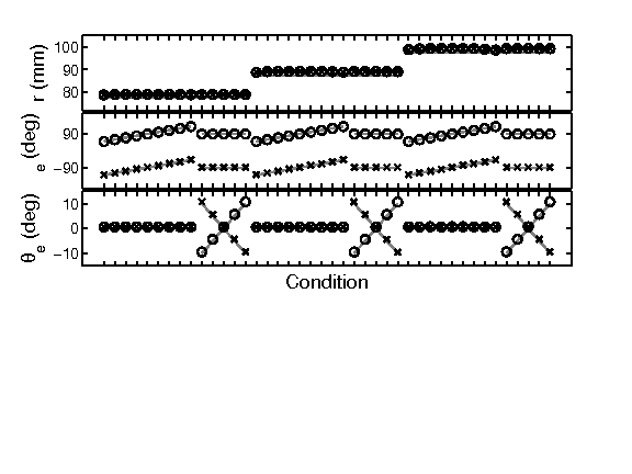
| 'fig5' | Reproduce Fig. 5: Estimated on-axis model parameters from HRTFs calculated for the centered object Sphere. Condition: combination of actual parameters used in HRTF simulation. Circle and cross: Parameters estimated for the left and right ears, respectively. Gray lines: Actual parameters. |
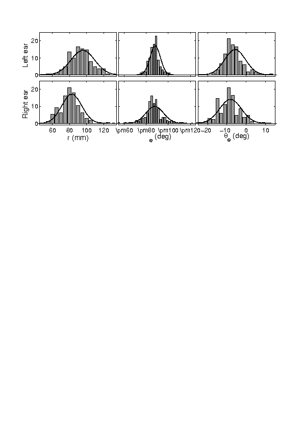
| 'fig6' | Reproduce Fig. 6: Estimated on-axis model parameters from left-ear (top row) and right-ear (bottom row) HRTFs of human listeners. Lines: normal distribution fitted to the data. phi_e: Positive and negative values corresponding to the left and right ears, respectively. |
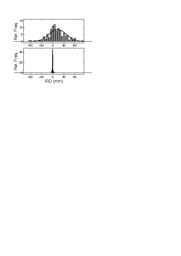
| 'fig7' | Reproduce Fig. 7: Estimated on-axis model IRDs from acoustically measured HRTFs of listeners. Line: normal distribution fitted to the data. |
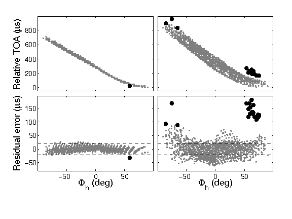
| 'fig8' | Reproduce Fig. 8: Relative TOAs (top row) and on-axis model fit residuals (bottom row) from HRTFs of STP (left column) and of an exemplary listener (NH89, ARI; right column). Black points: data classified as outliers by the ESD test with an upper bound of outlier rate of 1% (see ziegelwanger2014). The reference for the relative TOAs is the smallest TOA in each HRTF set. Horizontal lines: \(\pm1\) sampling interval. |
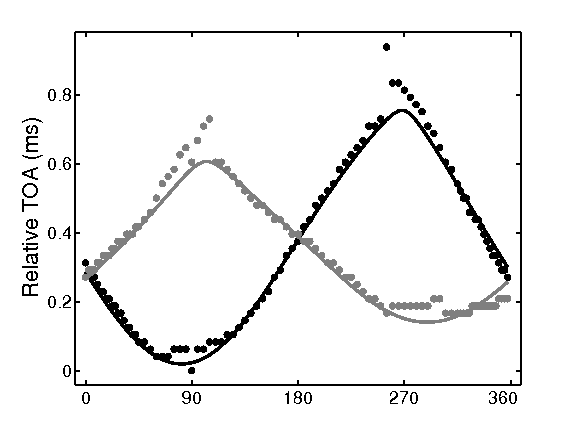
| 'fig9' | Reproduce Fig. 9: Relative TOAs of an exemplary listener (NH89, ARI) in the interaural horizontal plane for the left (black) and right (gray) ears as results from the MCM estimator (symbols) and the on-axis model (lines). The reference for the relative TOAs is the smallest TOA in HRTF sets of both ears. |
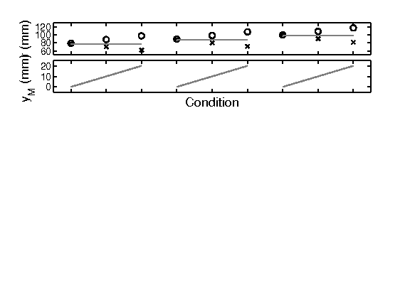
| 'fig10' | Reproduce Fig. 10: Estimated on-axis model parameters from HRTFs calculated for the non-centered object Sphere. Other details as in Fig. 5. |
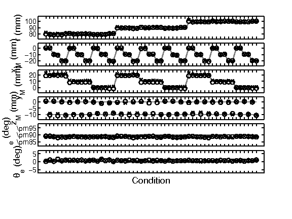
| 'fig12' | Reproduce Fig. 12: Estimated on-axis model parameters from HRTFs calculated for the non-centered object Sphere. Other details as in Fig. 5. phi_e: Positive and negative values correspond to the left and right ears, respectively. |
| 'tab1' | Reproduce Tab. 1: ANRs and parameter errors (average \(\pm1\) standard deviation) resulting from fitting the on-axis model to TOAs estimated from HRTFs of the Sphere. Parameter errors: Differences between the estimated and actual parameters. |
| 'tab2' | Reproduce Tab. 2: Parameters and ANRs resulting from fitting the on-axis model to TOAs estimated from HRTFs of the objects Sphere, SAT, STP. Actual parameters: r=87,5 mm, phi_e=90deg, and theta_e=0deg. |
| 'tab3' | Reproduce Tab. 3: Parameters (average \(\pm1\) standard deviation) and ANRs (median) resulting from fitting the on-axis model to TOAs estimated from acoustically measured HRTFs of human listeners. L: Left ear. R: Right ear. All: Results for all listeners. NH89: Results for a single listener (NH89, ARI). |
| 'tab5' | Reproduce Tab. 5: Parameters and ANRs (average \(\pm1\) standard deviation) resulting from fitting the off-axis model to TOAs estimated from HRTFs of SAT, STP, and all listeners (All). Full: Fits to full TOA sets. O-A: Fits to the outlier-adjusted TOA sets. L: Left ear. R: Right ear. |
| 'tab6' | Reproduce Tab. 6: ANRs and parameter errors (average \(\pm1\) standard deviation) resulting from fitting the off-axis model to TOAs estimated from HRTFs of the object Sphere. Centered: Conditions in which r and vec(e) varied from M=0. Non-centered: Conditions in which M varied. Other defails as in Tab. 5. |
Requirements:
- SOFA API from http://sourceforge.net/projects/sofacoustics for Matlab (in e.g. thirdparty/SOFA)
- Optimization Toolbox for Matlab
- Optional: Data in hrtf/ziegelwanger2014. Will be downloaded on demand.
Examples:
To display Fig. 3, use
exp_ziegelwanger2014('fig3');
To display Fig. 5, use
exp_ziegelwanger2014('fig5');
To display Fig. 6, use
exp_ziegelwanger2014('fig6');
To display Fig. 7, use
exp_ziegelwanger2014('fig7');
To display Fig. 8, use
exp_ziegelwanger2014('fig8');
To display Fig. 9, use
exp_ziegelwanger2014('fig9');
To display Fig. 10, use
exp_ziegelwanger2014('fig10');
To display Fig. 12, use
exp_ziegelwanger2014('fig12');
To display Tab. 1, use
exp_ziegelwanger2014('tab1');
This code produces the following output:
Tab. I.:
----------------------------------------------------------------------
EST || r error (mm) | phi_e error (deg) | theta_e errror |  ANR (----------------------------------------------------------------------
----------------------------------------------------------------------
MAX ||    2.9     0.2     1.1     0.1     0.8     0.0     6.5     0.1 CTD ||    3.2     0.2     1.2     0.1     0.9     0.1     7.0     0.2 AGD ||   15.4     1.0     1.9     0.1     2.5     0.0    23.6     0.6 MCM ||    1.6     0.2     1.1     0.1     0.6     0.0     6.1     0.1 ----------------------------------------------------------------------
To display Tab. 2, use
exp_ziegelwanger2014('tab2');
This code produces the following output:
Tab. II.:
----------------------------------------------------------------------------------------------------------
       ||     r error (mm)       |   phi_e error (deg)   |    theta_e errror     |       ANR (       || MAX | CTD | AGD  | MCM | MAX | CTD | AGD | MCM | MAX | CTD | AGD | MCM | MAX | CTD | AGD | MCM
----------------------------------------------------------------------------------------------------------
----------------------------------------------------------------------------------------------------------
Sphere || 91.5| 91.9| 104.7| 90.0| 89.9| 89.9| 89.3| 90.0|  0.4|  0.5|  1.7|  0.0|  6.1|  6.5| 19.4|  6.3
SAT    || 91.8| 92.7| 104.0| 90.1| 89.8| 89.7| 89.8| 89.8|  1.1|  1.6|  9.0|  0.7|  6.7|  8.8| 43.2|  6.5
STP    || 95.2| 95.0| 106.3| 93.1| 87.9| 87.8| 86.6| 88.4| -0.5| -0.5|  7.2| -0.2|  8.3|  8.5| 43.1|  8.5
----------------------------------------------------------------------------------------------------------
To display Tab. 3, use
exp_ziegelwanger2014('tab3');
This code produces the following output:
Tab. III.:
-----------------------------------------------------------------------
     | Ear || r (mm)       | phi_e (deg)  | theta_e (deg) |  ANR (-----------------------------------------------------------------------
-----------------------------------------------------------------------
All  |  L  ||  95.9   13.7   88.1    4.6   -5.6    5.3   42.3   51.2      |  R  ||  82.9   11.5  -87.7    8.0   -8.1    5.6   39.6   44.9 NH89 |  L  || 107.3    0.0   82.3    0.0   -7.8    0.0   29.9    0.0      |  R  ||  68.5    0.0  -72.6    0.0  -12.6    0.0   38.7    0.0 -----------------------------------------------------------------------
To display Tab. 5, use
exp_ziegelwanger2014('tab5');
This code produces the following output:
Tab. V.:
-------------------------------------------------------------------------------------------------------------------------------------------------
    | TOAset | Ear || r (mm)     | phi_e (deg) | theta_e (deg)| x_M (mm)    | y_M (mm)    | z_M (mm)    |  ANR (-------------------------------------------------------------------------------------------------------------------------------------------------
-------------------------------------------------------------------------------------------------------------------------------------------------
SAT |  Full  |  L  || 90.1   0.0  89.8   0.0   1.7   0.0   0.0   0.0   0.1   0.0  -2.0   0.0   6.4   0.0     |  Full  |  R  || 90.1   0.0  -89.8   0.0   1.7   0.0  -0.1   0.0  -0.1   0.0  -1.9   0.0   6.6   0.0     |  O-A   |  L  || 90.1   0.0  89.8   0.0   1.6   0.0   0.0   0.0   0.1   0.0  -1.9   0.0   6.4   0.0     |  O-A   |  R  || 90.1   0.0  -89.8   0.0   1.6   0.0  -0.1   0.0  -0.1   0.0  -1.8   0.0   6.6   0.0 STP |  Full  |  L  || 93.1   0.0  88.3   0.0  -0.1   0.0   0.7   0.0   0.0   0.0   0.9   0.0   8.9   0.0     |  Full  |  R  || 93.1   0.0  -88.2   0.0  -0.1   0.0   0.4   0.0  -0.0   0.0   0.8   0.0   9.1   0.0     |  O-A   |  L  || 93.1   0.0  88.3   0.0  -0.1   0.0   0.8   0.0   0.0   0.0   0.9   0.0   8.9   0.0     |  O-A   |  R  || 93.1   0.0  -88.2   0.0  -0.1   0.0   0.5   0.0  -0.0   0.0   0.8   0.0   9.1   0.0 ALL |  Full  |  L  || 92.1   6.4  85.2   8.4  -9.8  10.7  -4.7  12.5   7.6  14.7   7.6  17.8  40.5  50.4     |  Full  |  R  || 92.1   7.0  -83.3   9.9  -12.8   7.9  -6.6  13.0   6.9  18.4  10.4  14.6  37.3  44.4     |  O-A   |  L  || 91.1   6.3  85.2   9.2  -12.3   7.0  -4.3  12.8   7.4  13.7  11.0  12.8  29.0  12.9     |  O-A   |  R  || 91.1   6.5  -84.5   9.4  -13.9   7.4  -5.0  12.2   6.5  17.7  11.4  12.5  29.6  12.3 -------------------------------------------------------------------------------------------------------------------------------------------------
To display Tab. 6, use
exp_ziegelwanger2014('tab6');
This code produces the following output:
Tab. V.:
-------------------------------------------------------------------------------------------------------------------------------------------------
Condition    | TOAset | Ear || r error (mm) | phi_e error (deg) | theta_e errror | x_M error (mm) | y_M error (mm) | z_M error (mm) |  ANR (-------------------------------------------------------------------------------------------------------------------------------------------------
-------------------------------------------------------------------------------------------------------------------------------------------------
Centered     |  Full  |  L  ||    1.6     0.2    -1.2     0.3     0.9     0.6    -0.3     0.5     0.1     0.3    -0.4     0.9     6.2     0.1              |  Full  |  R  ||    1.6     0.2     1.3     0.4     0.8     0.6    -0.1     0.5    -0.1     0.2    -0.3     0.9     6.2     0.1              |  O-A   |  L  ||    1.6     0.2    -1.2     0.3     0.9     0.6    -0.3     0.5     0.1     0.3    -0.4     0.9     6.2     0.1              |  O-A   |  R  ||    1.6     0.2     1.3     0.4     0.8     0.6    -0.1     0.5    -0.1     0.2    -0.3     0.9     6.2     0.1 Non-centered |  Full  |  L  ||    2.2     0.6    -1.3     0.3     0.7     0.3    -0.1     0.4    -0.8     0.6    -0.0     0.5     6.2     0.1              |  Full  |  R  ||    2.6     0.8     1.3     0.3     0.6     0.3    -0.0     0.5     0.8     0.8     0.2     0.6     6.2     0.1              |  O-A   |  L  ||    2.3     0.5    -1.2     0.3     0.7     0.3     0.0     0.4    -0.9     0.5     0.0     0.5     6.2     0.1              |  O-A   |  R  ||    2.3     0.8     1.1     0.3     0.5     0.4     0.2     0.5     0.6     0.8     0.3     0.7     6.2     0.1 -------------------------------------------------------------------------------------------------------------------------------------------------
References:
H. Ziegelwanger and P. Majdak. Modeling the direction-continuous time-of-arrival in head-related transfer functions. J. Acoust. Soc. Am., 135:1278-1293, 2014.


Build with Bootstrap