THE AUDITORY MODELING TOOLBOX
This documentation page applies to an outdated major AMT version. We show it for archival purposes only.
Click here for the documentation menu and here to download the latest AMT (1.6.0).
EXP_LINDEMANN1986 - Figures from Lindemann (1986)
Usage
output = exp_lindemann1986(flag)
exp_lindemann1986(flag) reproduces the results for the figure given by flag from the Lindemann (1986) paper. It will also plot the results. The format of its output depends on the chosen figure. If not otherwise stated, the cross-correlation of a pure tone sinusoids with f=500 Hz and different ITDs, ILDs or a combination of both is calculated. Because of the stationary character of the input signals, \(T_{int} = \inf\) is used to produce only one time step in the crosscorr output.
The following flags can be specified;
| 'plot' | plot the output of the experiment. This is the default. |
| 'noplot' | Don't plot, only return data. |
| 'auto' | Re-calculate the file if it does not exist. Return 1 if the file exist, otherwise 0. This is the default |
| 'redo' | Always recalculate the results. |
| 'cached' | Always use the cached version. Default. |
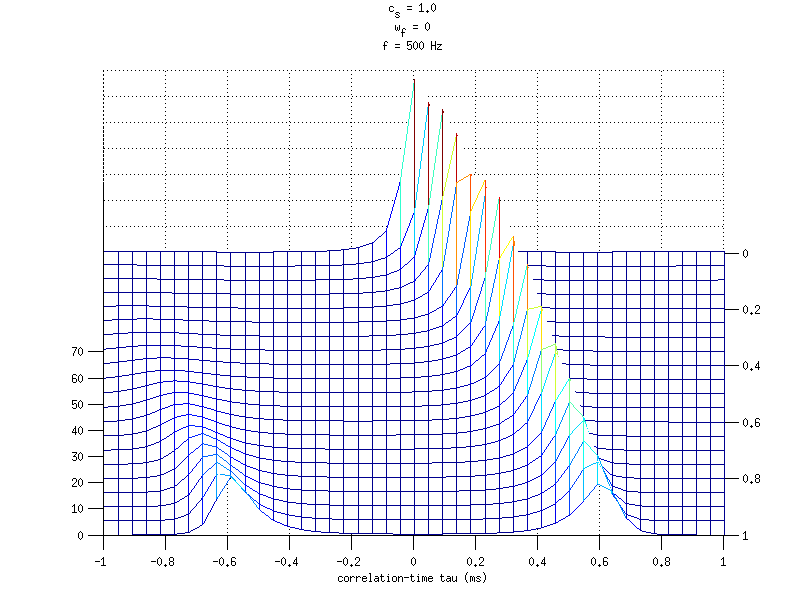
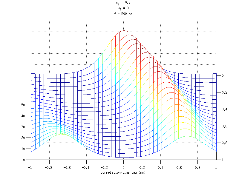
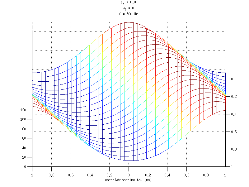
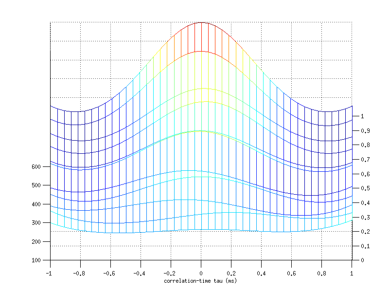
| 'fig6' | Reproduce Fig.6 from Lindemann (1986). The cross-correlation is calculated for different ITDs and different inhibition factors \(c_s=0,0.3,1\) . Afterwards for every c_s the correlation is plotted for every used ITD dependend on the correlation-time delay. The output is cross-correlation result of the figure. The output has dimensions: number of c_s conditions x nitds x delay line length |
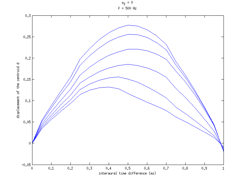
| 'fig7' | Reproduce Fig.7 from Lindemann (1986). The cross-correlation is calculated for different ITDs and different inhibition factors \(c_s=0,0.2,0.4,0.6,0.8,1.0\) . Afterwards for every c_s the displacement of the centroid of the auditory image is calculated and plotted depending on the ITD. The output is the displacement of the centroid for different c_s values. The output has dimensions: c_s x nitds |
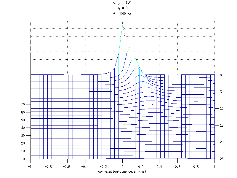
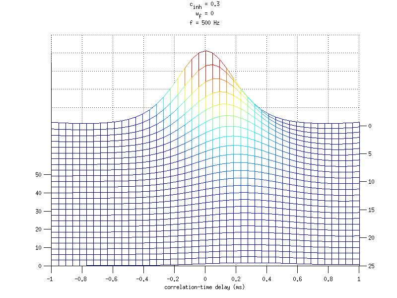
| 'fig8' | Reproduce Fig.8 from Lindemann (1986). The cross-correlation is calculated for different ILDs and different inhibition factors \(c_s = 0.3, 1\) . Afterwards for every c_s the ILD is plotted depending on the correlation time. The output is the cross-correlation result of the figure. The dimensions of the output are: number of c_s conditions x nilds x delay line length. |
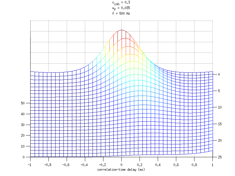
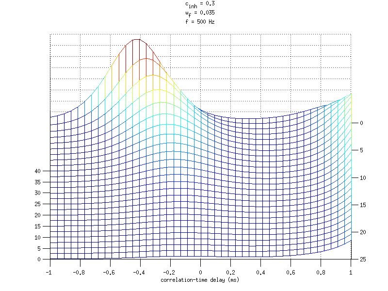
| 'fig10' | Reproduce Fig.10 from Lindemann (1986). The cross-correlation is calculated for different ILDs with an inhibition factor of \(c_s = 0.3\) and a monaural detector factor \(w_f = 0.035\) . Afterwards the ILD is plotted depending on the correlation time. The output is the cross-correlation result of the figure. The output has dimensions: number of c_s conditions x nilds x delay line length |
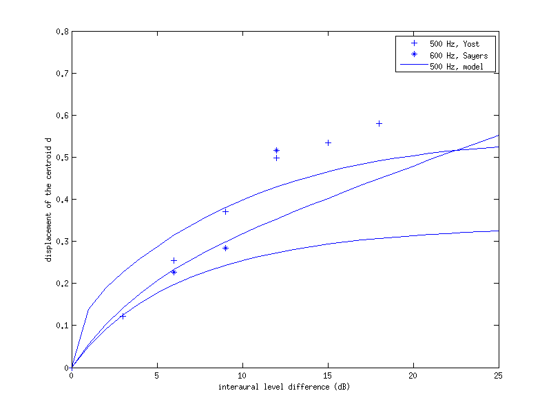
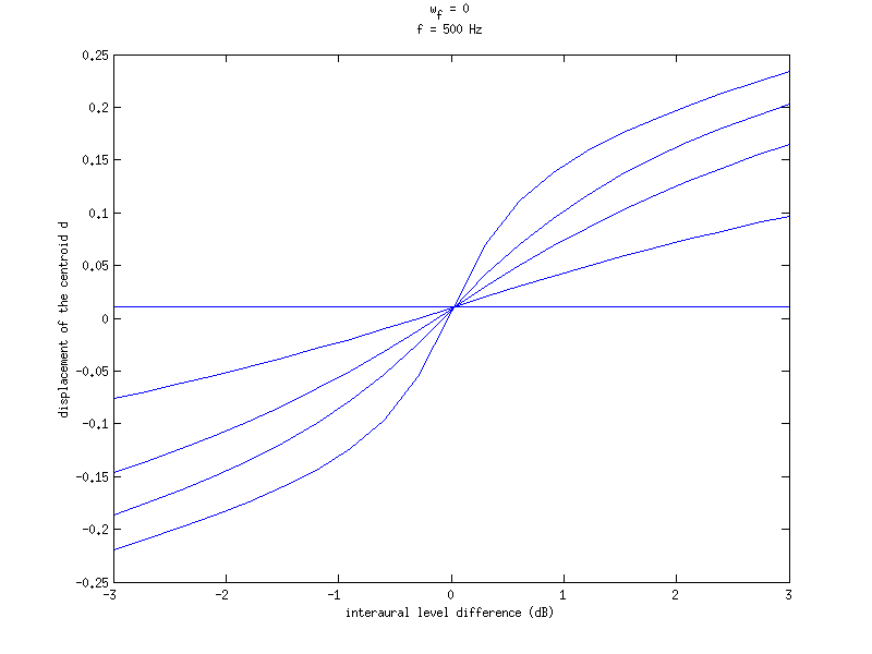
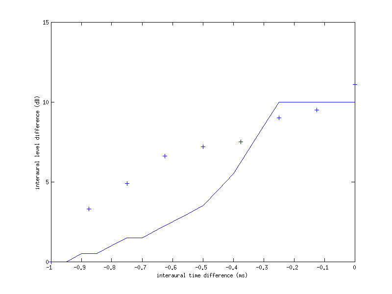
| 'fig11' | Reproduce Fig.11 from Lindemann (1986). The centroid position is calculated for different ILDs, an inhibition factor \(c_s = 0.3\) and a monaural detector factor 0.035 centroid is plotted dependend on the ILD. The output is the cross-correlation result of the to figure. The dimensions of the output are: number of c_s conditions x nilds x delay line length |
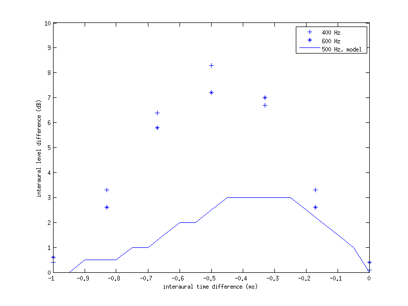
| 'fig12' | Reproduce Fig.12 from Lindemann (1986). The centroids are calculated for combinations of ITDs and ILDs. After the calculation the values for the centroids of the stimuli are searched to find the nearest value to 0. The corresponding ILD value is stored in output and plotted depending on the ITD. The output is the simulated results for a trading experiment. The ILD value for getting a centroid near the center for an combined ITD, ILD stimulus with a given ITD value. The output has dimensions: number of ITDs x 1 |
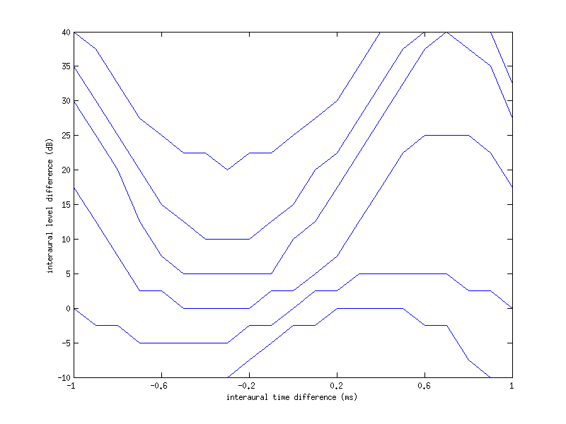
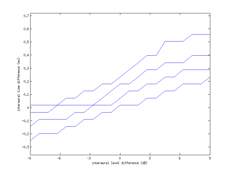
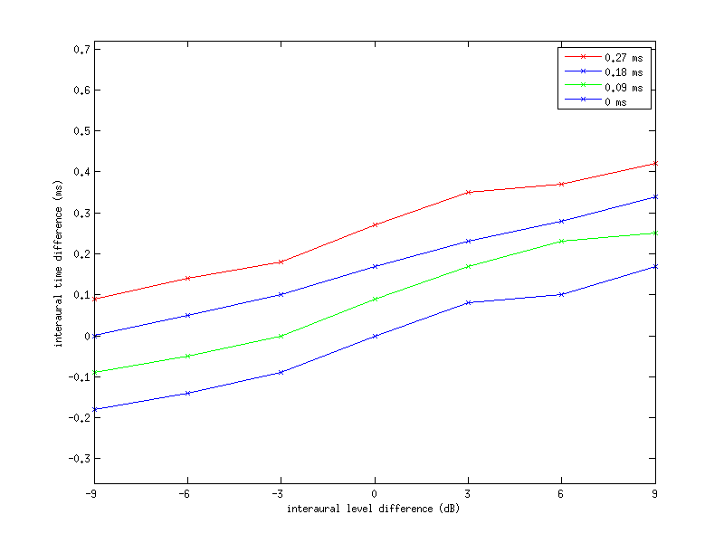
| 'fig13' | Reproduce Fig.13 from Lindemann (1986). The centroids are calculated for ILD only and ITD/ILD combination stimuli. After the calculation the values for the centroids of the ILD only stimuli are searched to find the nearest value to the centroid of a given combined stimulus. The resulting ILD value is stored for different combinaition values and plotted dependend on ITD. The output is the ILD value for getting the same lateralization with an ILD only stimulus compared to a stimulus with both ITD and ILD. The output has dimensions: number of ILDs x number of ITDs |
| 'fig14a' | Reproduce fig.14 (a) from Lindemann (1986). The cross-correlations for a combination of ILDs and a ITD of ~1ms are calculated. This is done for different ILDs and different inhibition factors \(c_s = 0,0.2,0.4,0.6,1\) . Afterwards for every c_s the centroid of the auditory image is calculated and plotted dependend on the ILD. The output is the displacement of the centroid for different c_s values and ILDs. The output has dimensions: c_s x nilds |
| 'fig14b' | Reproduce Fig.14 (b) from Lindemann (1986). The cross-correlations for a combination of ILDs and a ITD of ~1ms are calculated. This is done for different small ILDs with a standard deviation of 0-5. Afterwards for every standard deviation the mean centroid displacement is calculated and plotted dependend on the ITD. The output is the displacement of the centroid as a function of the ITD averaged over different small ILD with a standard deviation of \(0,1,2,3,4,5\) . The output has dimensions: nilds x nitds THIS FIGURE DOES NOT SEEM TO MATCH THE PAPER! |
| 'fig15' | Reproduce Fig.15 from Lindemann (1986). The cross-correlation for an ITD of -0.5ms is calculated. This is done for different ILDs, an inhibition factor \(c_s = 0.3\) and a monaural detector factor \(w_f = 0.035\) . Afterwards for every c_s the ILD is plotted depending on the correlation time. The output is the cross-correlation result. The output has dimensions: number of c_s conditions x nilds x delay line length |
| 'fig16' | Reproduces Fig.16 from Lindemann (1986). The cross-correlations for combinations of ITDs and ILDs are calculated. Afterwards the combinations of ILD and ITD are looked for the ones that have two peaks in its cross-correlation which have the nearly same height. The corresponding ILD value is than stored in output and plotted dependend on the ITD. The output is the ILD value for which the cross-correlation for a combined ITD, ILD stimulus has two peaks with the same (nearest) height, depending on the ITD. The output has dimensions: number of ITDs x 1 |
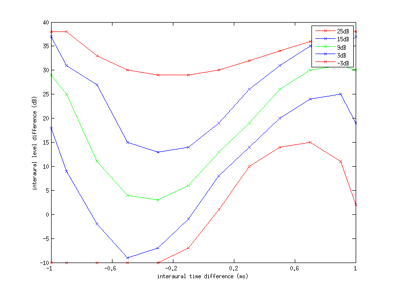
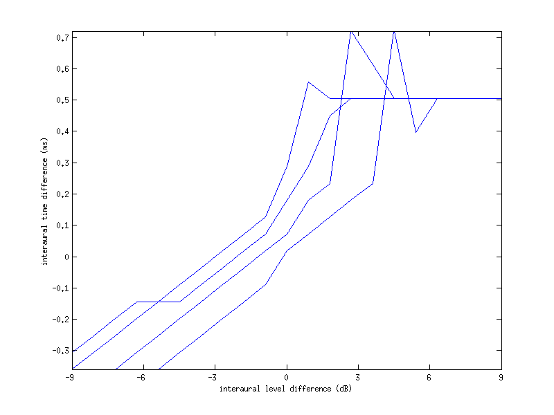
| 'fig17' | Reproduce Fig.17 from Lindemann (1986). The cross-correlation for ITD/ILD combination and ITD only stimuli is calculated. Afterwards the values for the centroids and maxima of the ITD only stimuli are searched to find the nearest value to the centroid and maxima of a given combined stimulus. The resulting ITD value is stored for different combinaition values. The output is the ITD value for getting the same lateralization with an ITD only stimulus compared to a stimulus with both ITD and ILD using the centroid of the cross-correlation. The output has dimensions: number of ITDs x number of ILDs. |
| 'fig18' | Reproduce Fig.18 from Lindemann (1986). The cross-correlation of pink noise with different interaural coherence values is calculated. Afterwards for every interaural coherence value the correlation is plotted dependend on the correlation-time delay. The output is the cross-correlation result of the figure. The output has dimensions: number of interaural coherences x delay line length |
If no flag is given, the function will print the list of valid flags.
Examples:
To display Figure 6 use
exp_lindemann1986('fig6');
To display Figure 7 use
exp_lindemann1986('fig7');
To display Figure 8 use
exp_lindemann1986('fig8');
To display Figure 10 use
exp_lindemann1986('fig10');
To display Figure 11 use
exp_lindemann1986('fig11');
To display Figure 12 use
exp_lindemann1986('fig12');
To display Figure 13 use
exp_lindemann1986('fig13');
To display Figure 14a use
exp_lindemann1986('fig14a');
To display Figure 15 use
exp_lindemann1986('fig15');
To display Figure 16 use
exp_lindemann1986('fig16');
To display Figure 17 use
exp_lindemann1986('fig17');
To display Figure 18 use
exp_lindemann1986('fig18');
References:
W. Lindemann. Extension of a binaural cross-correlation model by contralateral inhibition. I. Simulation of lateralization for stationary signals. J. Acoust. Soc. Am., 80:1608-1622, 1986.


Build with Bootstrap