THE AUDITORY MODELING TOOLBOX
This documentation page applies to an outdated major AMT version. We show it for archival purposes only.
Click here for the documentation menu and here to download the latest AMT (1.6.0).
EXP_BAUMGARTNER2014 - Results from Baumgartner et al. (2014)
Usage
data = exp_baumgartner2014(flag)
exp_baumgartner2014(flag) reproduces figures of the study from Baumgartner et al. (2014).
The following flags can be specified
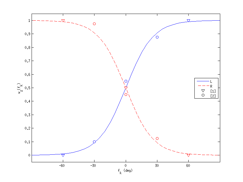
| 'fig2' | Reproduce Fig.2: Binaural weighting function best fitting results from Morimoto (2001) labeled as \([1]\) and Macpherson and Sabin (2007) labeled as \([2]\) in a least squared error sense. |
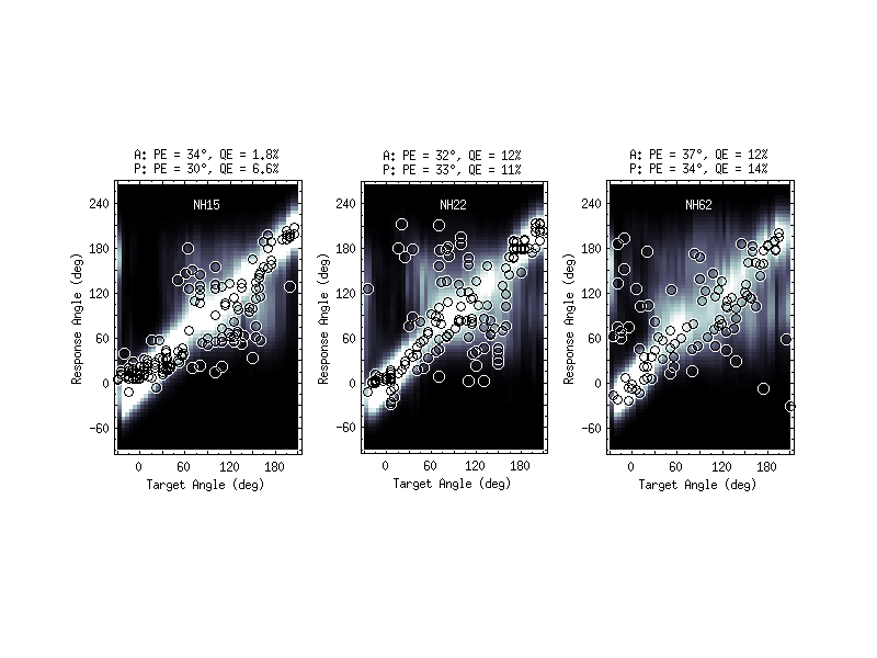
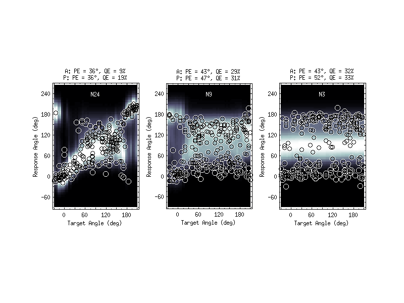
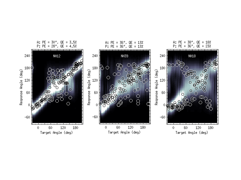
| 'fig3' | Reproduce Fig.3: Prediction examples. Actual responses and response predictions for three exemplary listeners when listening to median-plane targets in the baseline condition. Actual response angles are shown as open circles. Probabilistic response predictions are encoded by brightness according to the color bar to the right. Actual (A:) and predicted (P:) quadrant error rates (QE) and local polar RMS errors (PE) are listed above each panel. |
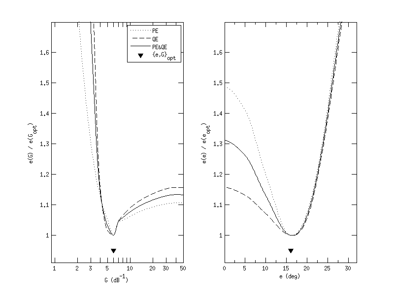
| 'fig4' | Reproduce Fig.4: Model parametrization. Partial and joint prediction residues as functions of the degree of selectivity and the motoric response scatter. Residuum functions are normalized to the minimum residuum obtained for the optimal parameter value. |
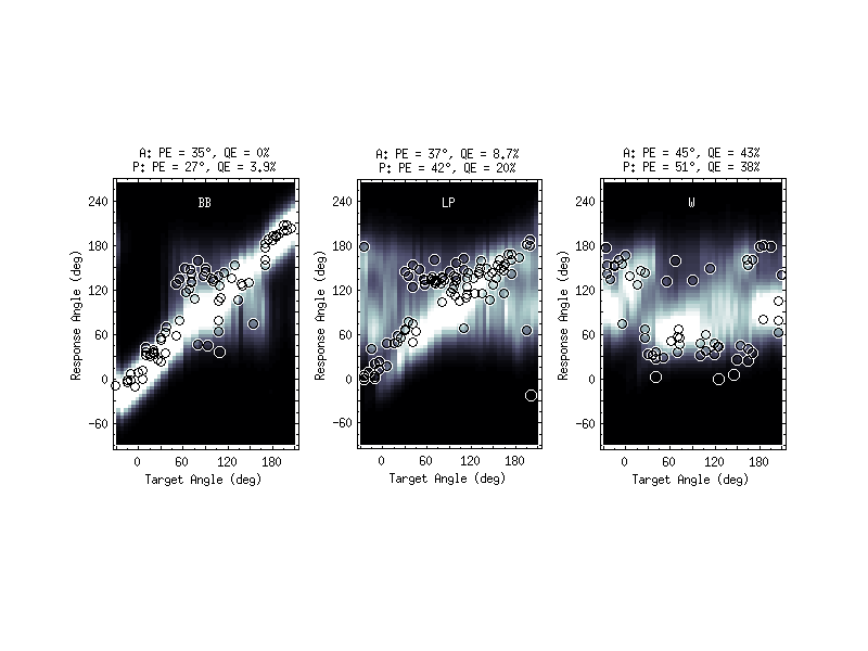
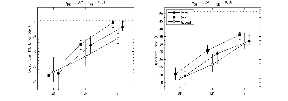
| 'fig5' | Reproduce Fig.5: Effect of band limitation and spectral warping. Actual responses and response predictions for listener NH12 when listening to broadband (BB), low-pass filtered (LP), or spectrally warped (W) DTFs of the median plane. Data were pooled within \(\pm15^\circ\) of lateral angle. All other conventions are as in Fig.3. |
| 'fig6' | Reproduce Fig.6: Effect of band limitation and spectral warping. Listeners were tested with broadband (BB), low-pass filtered (LP), and spectrally warped (W) DTFs. Actual: experimental results from Majdak et al. (2013). Part.: Model predictions for the actual eight participants based on the actually tested target positions. Pool: Model predictions for our listener pool based on all possible target positions. Symbols and whiskers show median values and inter-quartile ranges, respectively. Symbols were horizontally shifted to avoid overlaps. Dotted horizontal lines represent chance rate. Correlation coefficients, \(r\) , and prediction residues, \(e\) , specify the correspondence between actual and predicted listener-specific performances. |
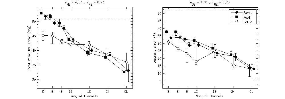
| 'fig7' | Reproduce Fig.7: Effect of spectral resolution in terms of varying the number of spectral channels of a channel vocoder. Actual responses and response predictions for exemplary listener NH12. Results for 24, 9, and 3 channels are shown. All other conventions are as in Fig.3. |
| 'fig8' | Reproduce Fig.8: Effect of spectral resolution in terms of varying the number of spectral channels of a channel vocoder. Actual experimental results are from Goupell et al. (2010). Stimulation with broadband click trains (CL) represents an unlimited number of channels. All other conventions are as in Fig.6. |
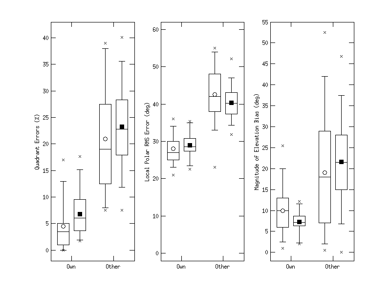
| 'fig9' | Reproduce Fig.9: Effect of non-individualized HRTFs in terms of untrained localization with others' instead of own ears. Statistics summaries with open symbols represent actual experimental results replotted from Fig.,13 of Middlebrooks (1999), statistics with filled symbols represent predicted results. Horizontal lines represent 25th, 50th, and 75th percentiles, the whiskers represent 5th and 95th percentiles, and crosses represent minima and maxima. Circles and squares denote mean values. |
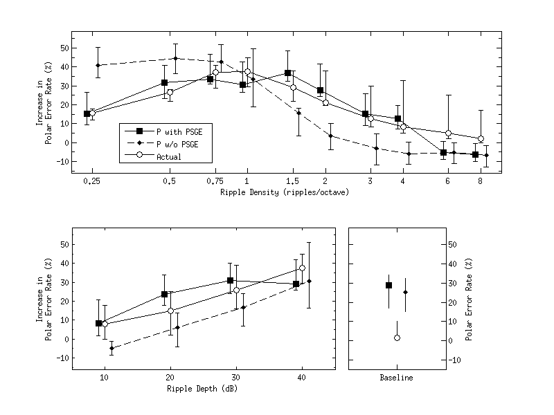
| 'fig10' | Reproduce Fig.10: Effect of spectral ripples. Actual experimental results (circles) are from Macpherson and Middlebrooks (2003). Predicted results (filled circles) were modeled for our listener pool (squares). Either the ripple depth of 40,dB (top) or the ripple density of one ripple/octave (bottom) was kept constant. Ordinates show the listener-specific difference in error rate between a test and the baseline condition. Baseline performances are shown in the bottom right panel. Symbols and whiskers show median values and inter-quartile ranges, respectively. Symbols were horizontally shifted to avoid overlaps. Diamonds with dashed lines show predictions (P) of the model without positive spectral gradient extraction (PSGE). |
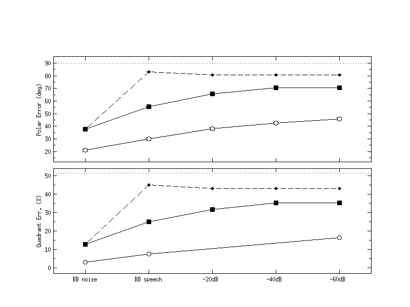
| 'fig11' | Reproduce Fig.11: Effect of high-frequency attenuation in speech localization. Actual experimental results are from Best et al. (2005). Absolute polar angle errors (top) and QE (bottom) were averaged across listeners. Circles and squares show actual and predicted results, respectively. Diamonds with dashed lines show predictions of the model without positive spectral gradient extraction. |
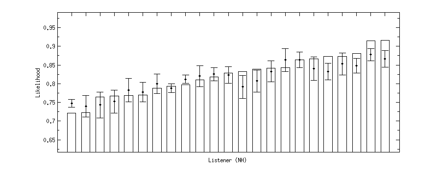
| 'fig12' | Reproduce Fig.12: Listener-specific likelihood statistics used to evaluate target-specific predictions for baseline condition. Bars show actual likelihoods, dots show mean expected likelihoods, and whiskers show tolerance intervals with 99% confidence level of expected likelihoods. |
| 'fig13' | Reproduce Fig.13: Exemplary baseline predictions. Same as Fig.3 but for listeners where actual likelihoods were outside the tolerance intervals. |
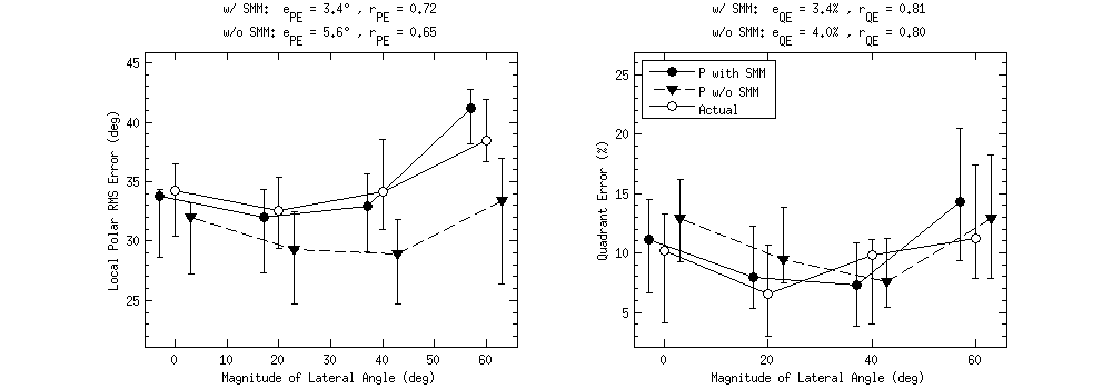
| 'fig14' | Reproduce Fig.14: Baseline performance as a function of the magnitude of the lateral response angle. Symbols and whiskers show median values and inter-quartile ranges, respectively. Open symbols represent actual and closed symbols predicted results. Symbols were horizontally shifted to avoid overlaps. Triangles with dashed lines show predictions (P) of the model without the sensomotoric mapping (SMM) stage. |
| 'tab1' | Reproduce Tab.1: Listener-specific sensitivity calibrated on the basis of N baseline targets in proximity of the median plane (+-30deg). Listeners are labeled as NH:math:l. Actual and predicted quadrant errors (QE) and local polar RMS errors (PE) are shown pairwise (Actual \(|\) Predicted). |
| 'tab2' | Reproduce Tab.2: The effects of model configurations on the prediction residues. PSGE: model with or without positive spectral gradient extraction. MBA: model with or without manual bandwidth adjustment to the stimulus bandwidth. Prediction residues between actual and predicted PE and QE are listed for acute performance with the broadband (BB), low-passed (LP) and warping (W) conditions of the experiments from Majdak et al. (2013). |
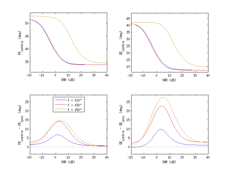
| 'tab3' | Reproduce Tab.3: Performance predictions for binaural, ipsilateral, and contralateral listening conditions. The binaural weighting coefficient was varied in order to represent the three conditions: binaural: \(\Phi = 13^\circ\) ; ipsilateral: \(\Phi \rightarrow +0^\circ\) ; contralateral: \(\Phi \rightarrow -0^\circ\) . Prediction residues and correlation coefficients between actual and predicted results are shown together with predicted average performances. |
| 'fig5_baumgartner2015aro' | |
| Reproduce Fig.5 of Baumgartner et al. (2015): Effect of background noise on reliability of contralateral cues for various lateral eccentricities. Top row: Across-listener averages of performance measures for contralateral ear. Bottom row: Contralateral re ipsilateral averages of performance measures. | |
| 'fig2_baumgartner2015jaes' | |
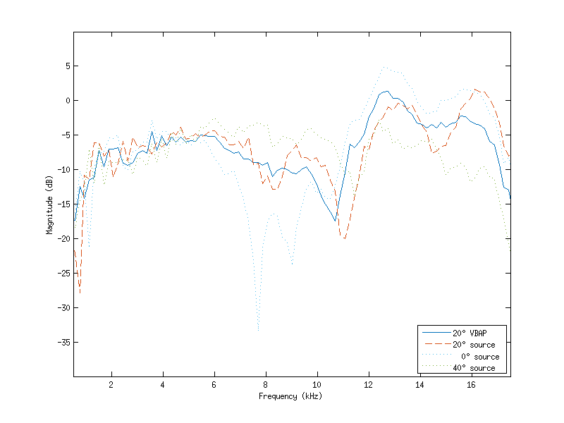
| Reproduce Fig.2 of Baumgartner and Majdak (2015): Example showing the spectral discrepancies obtained by VBAP. The targeted spectrum is the HRTF for 20 deg polar angle. The spectrum obtained by VBAP is the superposition of two HRTFs from directions 40 deg polar angle apart of each other with the tar- geted source direction centered in between. | |
| 'fig4_baumgartner2015jaes' | |
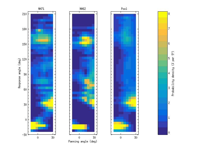
| Reproduce Fig.4 of Baumgartner and Majdak (2015): Response predictions to sounds created by VBAP with two loudspeakers in the median plane positioned at polar angles of -15 and 30 deg, respectively. Predictions for two exemplary listeners and pooled across all listeners. Each column of a panel shows the predicted PMV of polar-angle responses to a certain sound. Note the inter-individual differences and the generally small probabilities at response angles not occupied by the loudspeakers. | |
| 'fig5_baumgartner2015jaes' | |
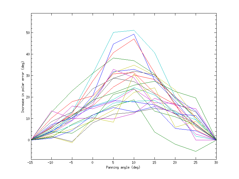
| Reproduce Fig.5 of Baumgartner and Majdak (2015): Listener-specific increases in polar error as a function of the panning angle. Increase in polar error defined as the difference between the polar error obtained by the VBAP source and the polar error obtained by the real source at the corresponding panning angle. Same loudspeaker arrangement as for Fig. 4. Note the large inter-individual differences and the increase in polar error being largest at panning angles centered between the loudspeakers, i.e., at panning ratios around R = 0 dB. | |
| 'fig6_baumgartner2015jaes' | |
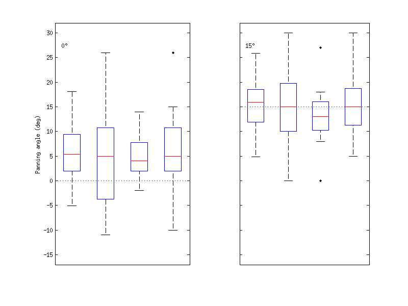
| Reproduce Fig.6 of Baumgartner and Majdak (2015): Panning angles for the loudspeaker arrangement of Fig. 4 judged best for reference sources at polar angles of 0 or 15 deg in the median plane. Comparison between experimental results from [2] and simulated results based on various response strategies: PM, CM, and both mixed. Dotted horizontal line: polar angle of the reference source. Hor- izontal line within box: median; box: inter-quartile range (IQR); whisker: within quartile \(\pm 1.5\) IQR; star: outlier. Note that the simulations predicted a bias similar to the results from Pulkki (2001) for the reference source at 0 deg. | |
| 'tab1_baumgartner2015jaes' | |
| Reproduce Tab.1 of Baumgartner and Majdak (2015): Means and standard deviations of responded panning angles for the two reference sources (Ref.) together with corresponding GOFs evaluated for the actual results from Pulkki (2001) and predicted results based on various response strategies. Note the relatively large GOFs for the simulations based on mixed response strategies indicating a good correspondence between actual and predicted results. | |
| 'fig7_baumgartner2015jaes' | |
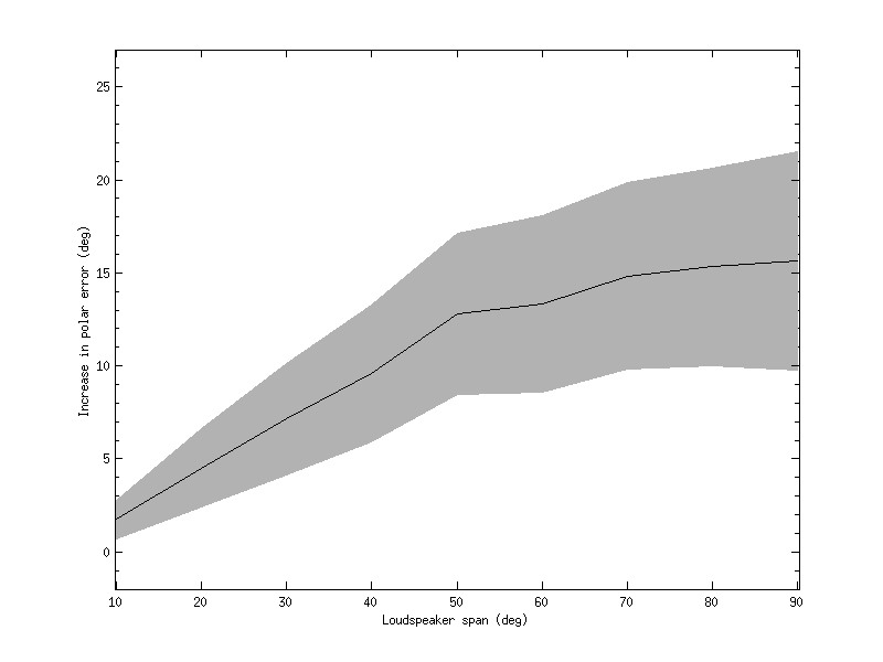
| Reproduce Fig.7 of Baumgartner and Majdak (2015): Increase in polar error (defined as in Fig. 5) as a function of loudspeaker span in the median plane with panning ratio R = 0 dB. Black line with gray area indicates mean \(\pm 1\) standard deviation across listeners. Note that the increase in polar error monotonically increases with loudspeaker span. | |
| 'fig8_baumgartner2015jaes' | |
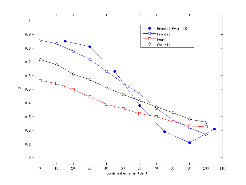
| Reproduce Fig.8 of Baumgartner and Majdak (2015): Effect of loudspeaker span in the median plane on coefficient of determination, r^2, for virtual source directions created by VBAP. Separate analysis for frontal, rear, and overall (frontal and rear) targets. Data pooled across listeners. Note the correspondence with the results obtained by Bremen et al. (2010). | |
| 'tab3_baumgartner2015jaes' | |
| Reproduce Tab.3 of Baumgartner and Majdak (2015): Predicted across-listener average of increase in polar errors as referred to a reference system containing loudspeakers at all considered directions. Distinction between mean and maximum degradation across directions. N: Number of loudspeakers. Ele.: Elevation of second layer. Notice that this elevation has a larger effect on mean and maximum degradation than N. | |
| 'fig9_baumgartner2015jaes' | |
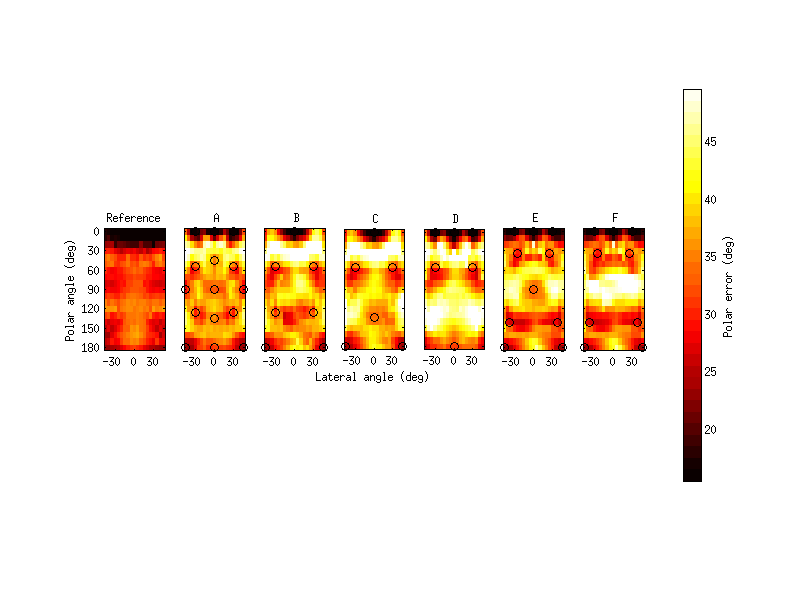
| Reproduce Fig.9 of Baumgartner and Majdak (2015): Predicted polar error as a function of the lateral and polar angle of a virtual source created by VBAP in various multichannel systems. Open circles indicate loudspeaker directions. Reference shows polar error predicted for a real source placed at the virtual source directions investigated for systems A, ..., F. | |
Further, cache flags (see amt_cache) and plot flags can be specified:
| 'plot' | Plot the output of the experiment. This is the default. |
| 'noplot' | Don't plot, only return data. |
Requirements:
- SOFA API v0.4.3 or higher from http://sourceforge.net/projects/sofacoustics for Matlab (in e.g. thirdparty/SOFA)
- Data in hrtf/baumgartner2014
- Statistics Toolbox for Matlab (for some of the figures)
Examples:
To display Fig.2 use
exp_baumgartner2014('fig2');
This code produces the following output:
Phi: 13 deg
To display Fig.3 use
exp_baumgartner2014('fig3');
To display Fig.4 use
exp_baumgartner2014('fig4');
This code produces the following output:
Optimal Gamma: 6 dB^-1
Optimal MRS: 16 deg
To display Fig.5 use
exp_baumgartner2014('fig5');
This code produces the following output:
Listener: NH12
To display Fig.6 use
exp_baumgartner2014('fig6');
To display Fig.7 use
exp_baumgartner2014('fig7');
This code produces the following output:
Listener: NH12
To display Fig.8 use
exp_baumgartner2014('fig8');
To display Fig.9 use
exp_baumgartner2014('fig9');
To display Fig.10 use
exp_baumgartner2014('fig10');
This code produces the following output:
Correlation between actual and predicted median values (15 conditions):
w/  PSGE: r = 0.88
w/o PSGE: r = 0.78
To display Fig.11 use
exp_baumgartner2014('fig11');
To display Fig.12 use
exp_baumgartner2014('fig12');
To display Fig.13 use
exp_baumgartner2014('fig13');
To display Fig.14 use
exp_baumgartner2014('fig14');
To display Fig.5 of Baumgartner et al. (2015) use
exp_baumgartner2014('fig5_baumgartner2015aro');
To display Fig.2 of Baumgartner and Majdak (2015) use
exp_baumgartner2014('fig2_baumgartner2015jaes');
To display Fig.4 of Baumgartner and Majdak (2015) use
exp_baumgartner2014('fig4_baumgartner2015jaes');
To display Fig.5 of Baumgartner and Majdak (2015) use
exp_baumgartner2014('fig5_baumgartner2015jaes');
To display Fig.6 of Baumgartner and Majdak (2015) use
exp_baumgartner2014('fig6_baumgartner2015jaes');
To display Fig.7 of Baumgartner and Majdak (2015) use
exp_baumgartner2014('fig7_baumgartner2015jaes');
To display Fig.8 of Baumgartner and Majdak (2015) use
exp_baumgartner2014('fig8_baumgartner2015jaes');
To display Fig.9 of Baumgartner and Majdak (2015) use
exp_baumgartner2014('fig9_baumgartner2015jaes');
To display Tab.1 of Baumgartner and Majdak (2015) use
exp_baumgartner2014('tab1_baumgartner2015jaes');
This code produces the following output:
p-values of K.S.-test:
Real source at 0 deg:
Results Pulkki (2001): p = 0.77
Probability Maximiz.:  p = 0.01
Centroid Match:        p = 0.42
Individual strategy:   p = 0.88 (#CM = 11)
Real source at 15 deg:
Results Pulkki (2001): p = 0.70
Probability Maximi.:   p = 0.37
Centroid Match:        p = 0.02
Individual strategy:   p = 0.84 (#CM = 11)
To display Tab.3 of Baumgartner and Majdak (2015) use
exp_baumgartner2014('tab3_baumgartner2015jaes');
This code produces the following output:
RMS error difference from reference averaged across directions
System  min  mean  max
\it A -7.0 6.7 28.8
\it B -7.3 8.9 38.6
\it C -2.9 10.0 38.6
\it D -2.6 11.0 31.3
\it E -7.3 6.4 29.3
\it F -6.5 7.3 29.3


bremen2010pinna goupell2010numchan macpherson2007 macpherson2003ripples
majdak2013spatstrat middlebrooks1999nonindividualized morimoto2001
pulkki2001localization
References:
R. Baumgartner, P. Majdak, and B. Laback. The reliability of contralateral spectral cues for sound localization in sagittal planes. In Midwinter Meeting of the Association for Research in Otolaryngology, Baltimore, MD, Feb 2015.
R. Baumgartner, P. Majdak, and B. Laback. Modeling sound-source localization in sagittal planes for human listeners. The Journal of the Acoustical Society of America, 136(2):791-802, 2014. [ DOI ]
R. Baumgartner and P. Majdak. Modeling Localization of Amplitude-Panned Virtual Sources in Sagittal Planes. J. Audio Eng. Soc., 63(7/8):562-569, Aug. 2015. [ DOI | http ]


Build with Bootstrap