THE AUDITORY MODELING TOOLBOX
This documentation page applies to an outdated AMT version (1.0.0). Click here for the most recent page.
EXP_BAUMGARTNER2014 - Results from Baumgartner et al. (2014)
Usage
data = exp_baumgartner2014(flag)
Description
exp_baumgartner2014(flag) reproduces figures of the study from Baumgartner et al. (2014).
The following flags can be specified
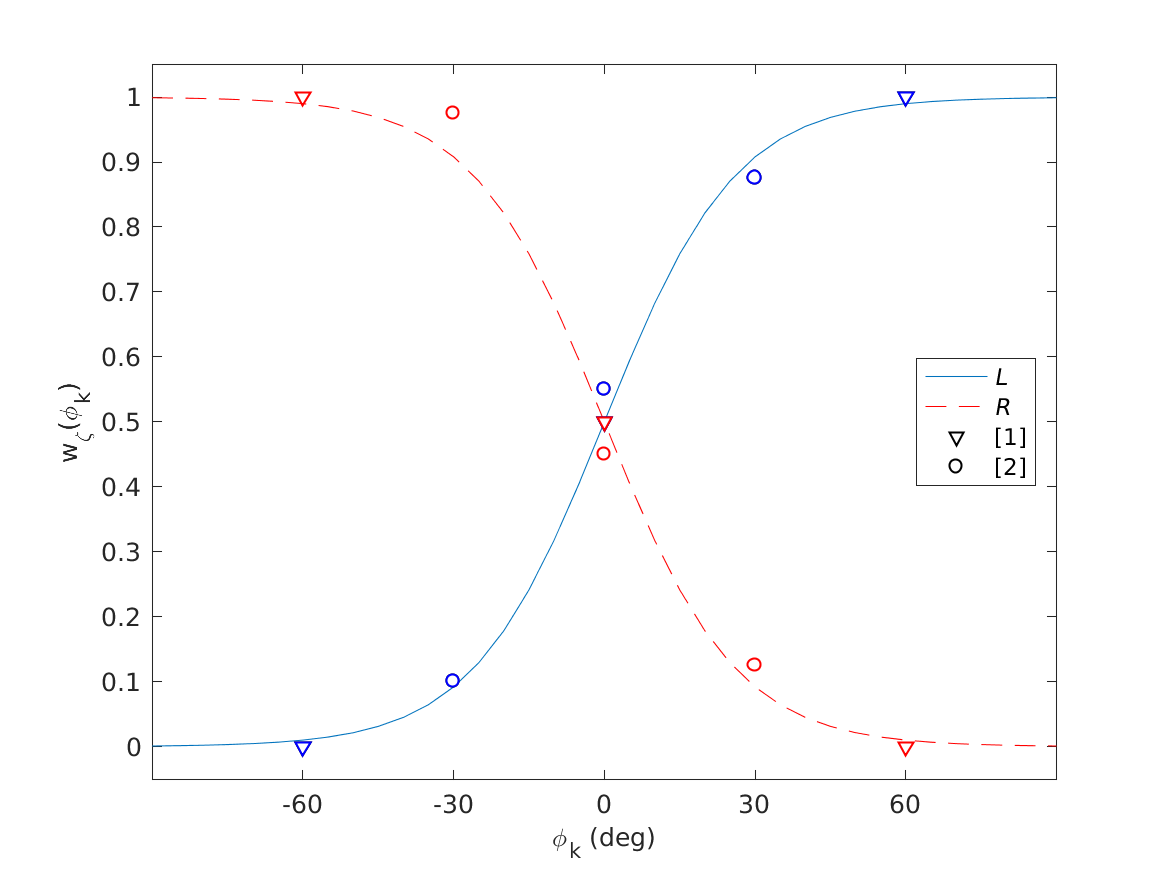
| 'fig2' | Reproduce Fig.2: Binaural weighting function best fitting results from Morimoto (2001) labeled as \([1]\) and Macpherson and Sabin (2007) labeled as \([2]\) in a least squared error sense. |
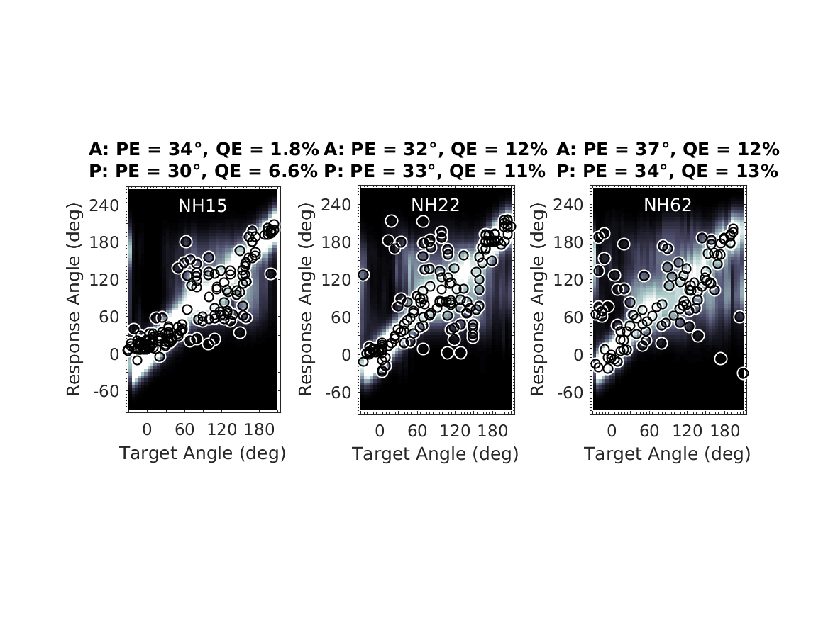
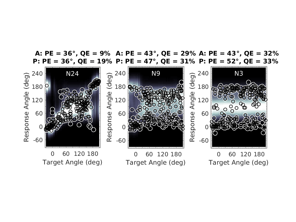
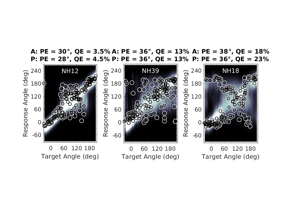
| 'fig3' | Reproduce Fig.3: Prediction examples. Actual responses and response predictions for three exemplary listeners when listening to median-plane targets in the baseline condition. Actual response angles are shown as open circles. Probabilistic response predictions are encoded by brightness according to the color bar to the right. Actual (A:) and predicted (P:) quadrant error rates (QE) and local polar RMS errors (PE) are listed above each panel. |
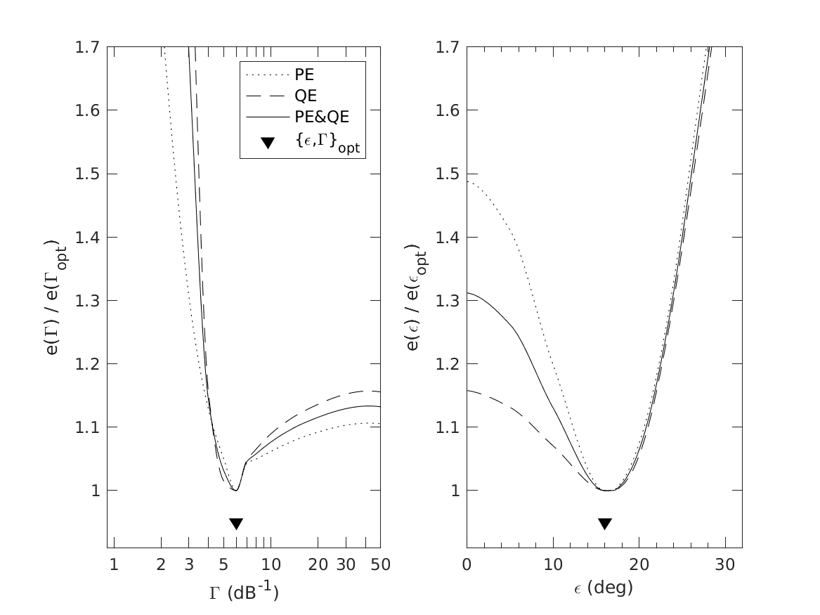
| 'fig4' | Reproduce Fig.4: Model parametrization. Partial and joint prediction residues as functions of the degree of selectivity and the motoric response scatter. Residuum functions are normalized to the minimum residuum obtained for the optimal parameter value. |
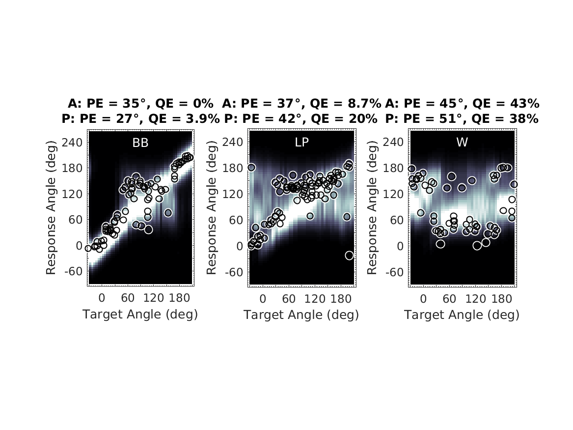
| 'fig5' | Reproduce Fig.5: Effect of band limitation and spectral warping. Actual responses and response predictions for listener NH12 when listening to broadband (BB), low-pass filtered (LP), or spectrally warped (W) DTFs of the median plane. Data were pooled within \(\pm15^\circ\) of lateral angle. All other conventions are as in Fig.3. |
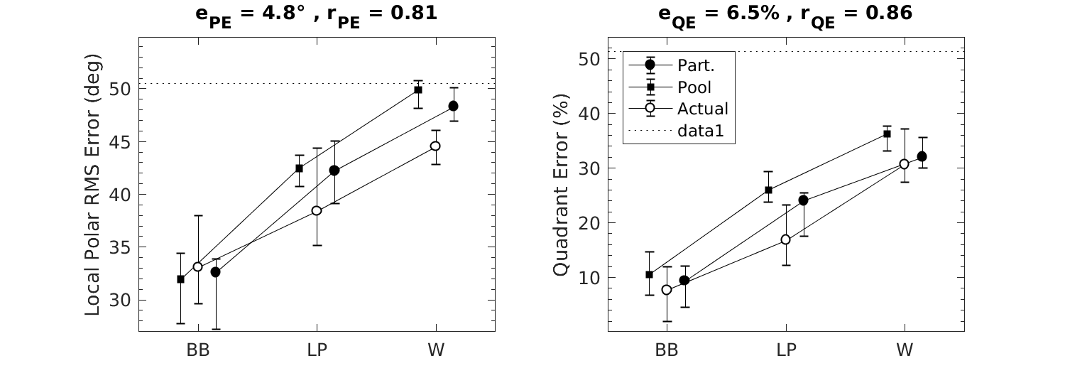
| 'fig6' | Reproduce Fig.6: Effect of band limitation and spectral warping. Listeners were tested with broadband (BB), low-pass filtered (LP), and spectrally warped (W) DTFs. Actual: experimental results from Majdak et al. (2013). Part.: Model predictions for the actual eight participants based on the actually tested target positions. Pool: Model predictions for our listener pool based on all possible target positions. Symbols and whiskers show median values and inter-quartile ranges, respectively. Symbols were horizontally shifted to avoid overlaps. Dotted horizontal lines represent chance rate. Correlation coefficients, \(r\), and prediction residues, \(e\), specify the correspondence between actual and predicted listener-specific performances. |
| 'fig7' | Reproduce Fig.7: Effect of spectral resolution in terms of varying the number of spectral channels of a channel vocoder. Actual responses and response predictions for exemplary listener NH12. Results for 24, 9, and 3 channels are shown. All other conventions are as in Fig.3. |
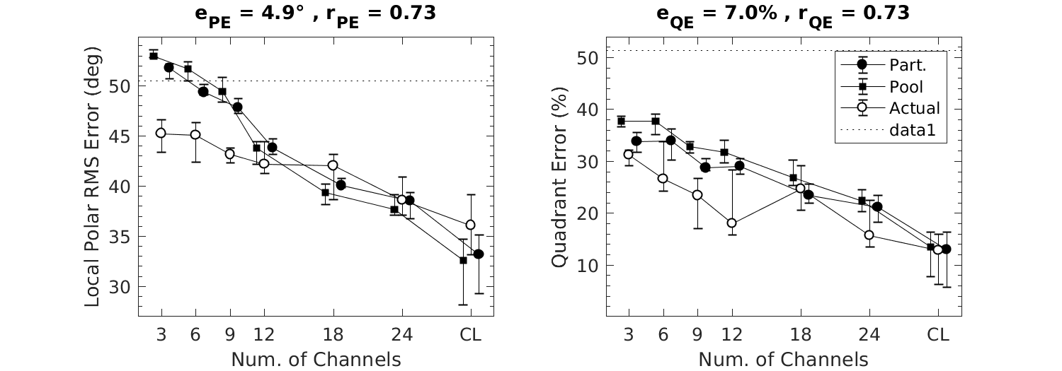
| 'fig8' | Reproduce Fig.8: Effect of spectral resolution in terms of varying the number of spectral channels of a channel vocoder. Actual experimental results are from Goupell et al. (2010). Stimulation with broadband click trains (CL) represents an unlimited number of channels. All other conventions are as in Fig.6. |
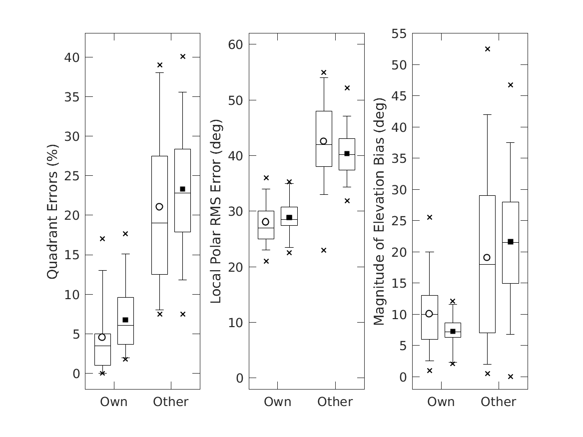
| 'fig9' | Reproduce Fig.9: Effect of non-individualized HRTFs in terms of untrained localization with others' instead of own ears. Statistics summaries with open symbols represent actual experimental results replotted from Fig.,13 of Middlebrooks (1999), statistics with filled symbols represent predicted results. Horizontal lines represent 25th, 50th, and 75th percentiles, the whiskers represent 5th and 95th percentiles, and crosses represent minima and maxima. Circles and squares denote mean values. Dimensions of |
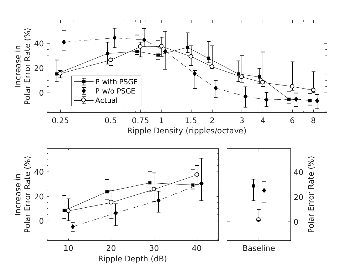
| 'fig10' | Reproduce Fig.10: Effect of spectral ripples. Actual experimental results (circles) are from Macpherson and Middlebrooks (2003). Predicted results (filled circles) were modeled for our listener pool (squares). Either the ripple depth of 40,dB (top) or the ripple density of one ripple/octave (bottom) was kept constant. Ordinates show the listener-specific difference in error rate between a test and the baseline condition. Baseline performances are shown in the bottom right panel. Symbols and whiskers show median values and inter-quartile ranges, respectively. Symbols were horizontally shifted to avoid overlaps. Diamonds with dashed lines show predictions (P) of the model without positive spectral gradient extraction (PSGE). |
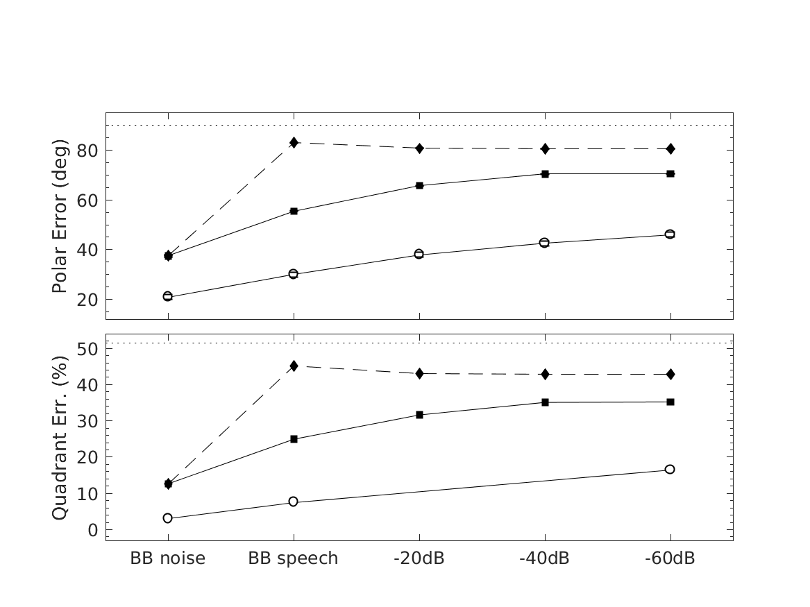
| 'fig11' | Reproduce Fig.11: Effect of high-frequency attenuation in speech localization. Actual experimental results are from Best et al. (2005). Absolute polar angle errors (top) and QE (bottom) were averaged across listeners. Circles and squares show actual and predicted results, respectively. Diamonds with dashed lines show predictions of the model without positive spectral gradient extraction. |
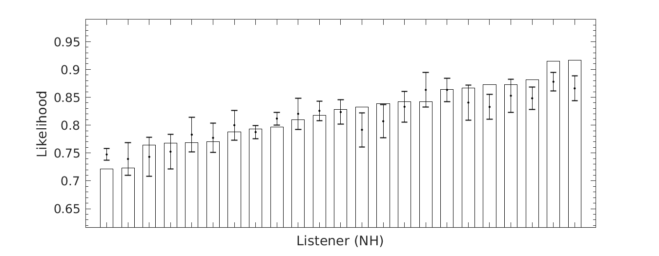
| 'fig12' | Reproduce Fig.12: Listener-specific likelihood statistics used to evaluate target-specific predictions for baseline condition. Bars show actual likelihoods, dots show mean expected likelihoods, and whiskers show tolerance intervals with 99% confidence level of expected likelihoods. |
| 'fig13' | Reproduce Fig.13: Exemplary baseline predictions. Same as Fig.3 but for listeners where actual likelihoods were outside the tolerance intervals. |
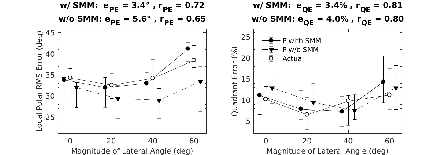
| 'fig14' | Reproduce Fig.14: Baseline performance as a function of the magnitude of the lateral response angle. Symbols and whiskers show median values and inter-quartile ranges, respectively. Open symbols represent actual and closed symbols predicted results. Symbols were horizontally shifted to avoid overlaps. Triangles with dashed lines show predictions (P) of the model without the sensomotoric mapping (SMM) stage. |
| 'tab1' | Reproduce Tab.1: Listener-specific sensitivity calibrated on the basis of N baseline targets in proximity of the median plane (+-30deg). Listeners are labeled as NH:math:l. Actual and predicted quadrant errors (QE) and local polar RMS errors (PE) are shown pairwise (Actual \(|\) Predicted). |
| 'tab2' | Reproduce Tab.2: The effects of model configurations on the prediction residues. PSGE: model with or without positive spectral gradient extraction. MBA: model with or without manual bandwidth adjustment to the stimulus bandwidth. Prediction residues between actual and predicted PE and QE are listed for acute performance with the broadband (BB), low-passed (LP) and warping (W) conditions of the experiments from Majdak et al. (2013). |
| 'tab3' | Reproduce Tab.3: Performance predictions for binaural, ipsilateral, and contralateral listening conditions. The binaural weighting coefficient was varied in order to represent the three conditions: binaural: \(\Phi = 13^\circ\); ipsilateral: \(\Phi \rightarrow +0^\circ\); contralateral: \(\Phi \rightarrow -0^\circ\). Prediction residues and correlation coefficients between actual and predicted results are shown together with predicted average performances. |
Further, cache flags (see amt_cache) and plot flags can be specified:
| 'plot' | Plot the output of the experiment. This is the default. |
| 'no_plot' | Don't plot, only return data. |
Requirements:
- SOFA API v0.4.3 or higher from http://sourceforge.net/projects/sofacoustics for Matlab (in e.g. thirdparty/SOFA)
- Data in hrtf/baumgartner2014
- Statistics Toolbox for Matlab (for some of the figures)
Examples:
To display Fig.2 use
exp_baumgartner2014('fig2');
This code produces the following output:
Phi: 13 deg
To display Fig.3 use
exp_baumgartner2014('fig3');
To display Fig.4 use
exp_baumgartner2014('fig4');
This code produces the following output:
Optimal Gamma: 6 dB^-1
Optimal MRS: 16 deg
To display Fig.5 use
exp_baumgartner2014('fig5');
This code produces the following output:
Listener: NH12
To display Fig.6 use
exp_baumgartner2014('fig6');
To display Fig.7 use
exp_baumgartner2014('fig7');
This code produces the following output:
Listener: NH12
To display Fig.8 use
exp_baumgartner2014('fig8');
To display Fig.9 use
exp_baumgartner2014('fig9');
To display Fig.10 use
exp_baumgartner2014('fig10');
This code produces the following output:
Correlation between actual and predicted median values (15 conditions):
w/  PSGE: r = 0.88
w/o PSGE: r = 0.78
To display Fig.11 use
exp_baumgartner2014('fig11');
To display Fig.12 use
exp_baumgartner2014('fig12');
To display Fig.13 use
exp_baumgartner2014('fig13');
To display Fig.14 use
exp_baumgartner2014('fig14');
References:
R. Baumgartner, P. Majdak, and B. Laback. The reliability of contralateral spectral cues for sound localization in sagittal planes. In Midwinter Meeting of the Association for Research in Otolaryngology, Baltimore, MD, Feb 2015.
R. Baumgartner, P. Majdak, and B. Laback. Modeling sound-source localization in sagittal planes for human listeners. The Journal of the Acoustical Society of America, 136(2):791--802, 2014. [ DOI ]
R. Baumgartner and P. Majdak. Modeling Localization of Amplitude-Panned Virtual Sources in Sagittal Planes. J. Audio Eng. Soc., 63(7/8):562--569, Aug. 2015. [ DOI | http ]


