THE AUDITORY MODELING TOOLBOX
This documentation page applies to an outdated AMT version (1.2.0). Click here for the most recent page.
EXP_BARUMERLI2022 - Experiments and results of Barumerli et al. (2022)
Usage
[] = exp_barumerli2022(flag)
Description
exp_barumerli2022(flag) reproduces figures and results of the study from Barumerli et al. (2021).
The following flags can be specified
| 'tab2' | Report data in Tab.2: The metrics LE, PE and QE computed for each fitted model are compared to the actual performances of five listeners in Majdak et al. (2010). Three different versions are tested each one with a different features space. The first considers with only binaural cues, the second combines binaural cues with spectral amplitudes and the third relies on binaural cues and spectral gradients. |
| 'gain_test' | Report results on prior contribution: This experiment prints the results of the analysis which employs the polar gain metric as in Ege et al. (2018) to quantify the contribution of the prior distribution. |
| 'fig3' | Reproduce Fig.3: Binarual feature examples. Visual comparison between the interaural cues for one subject in the frontal and horizontal plane. |
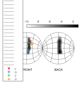
| 'fig4' | Reproduce Fig.4: Monaural feature examples. Visual comparison between the spectral cues for one subject in the median plane. |
| 'fig5' | Reproduce Fig.5: Prediction examples. Example of the model inferring the sound direction. Particularly, the plot shows the prediction of the bayesian observer based on the posterior distribution. Finally, such estimate is corrupted by motor noise required by the listener to provide a response. |
| 'fig6' | Reproduce Fig.6: Example of the fitted model based on spectral gradients. The actual data for both lateral and polar dimensions are from subject NH16 from Majdak et al. (2010). Moreover, model predictions, black dots, are: (a) based only on the likelihood function (i.e. inference driven only by sensory evidence) as in Reijniers et al. (2014) (b) Bayesian inference with both prior belief and sensory evidence. (c) Full model (i.e. Bayesian inference and sensorimotor stage. |
| 'fig7' | Reproduce Fig.7: Comparison between fitted models and actual data for five listeners in Majdak et al (2010). Actual (gray) and predicted (black) are the sound-localization performance metrics obtained by models based on spectral amplitues or gradients. Each row reports a different metrics: the first is about the Lateral Error (LE) as function of the lateral angle, the second and the third show the Polar Error (PE) and Quadrant Error (QE), respectively as a function of the polar angle, calculated for all targets within the lateral interval [-30, 30]deg. |
| 'fig8' | Reproduce Fig.8: see flag exp_middlebrooks1999 |
| 'fig9' | Reproduce Fig.9: see flag exp_macpherson2003 |
| 'exp_middlebrooks1999' | |
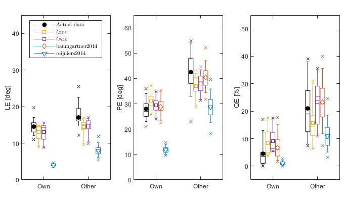
| Reproduce Fig.7: Predicted localization performance obtained for the individual (Own) and non-individual (Other) HRTFs with models based on two feature spaces. Additionally, predictions from Reijniers et al. (2014) and Baumgartner et al. (2014) as well as actual data from the original experiment Middlebrooks (1999) are shown. | |
| 'exp_macpherson2003' | |
| Reproduce Fig.8: Effect of the spectral ripples on sound localization performance by means of the polar error metric. Top and bottom left panels show differences to the reference condition in the right-most bottom panel which reports the polar errors obtained with broadband noise without spectral ripples. All panels show, in addition to predictions from our models, predictions from Reijniers et al (2014) and Baumgartner et al. (2014) as well as actual data from the original experiment Macpherson and Middlebrooks (2003). | |
Further, cache flags (see amt_cache) and plot flags can be specified:
| 'plot' | Plot the output of the experiment. This is the default. |
| 'no_plot' | Don't plot, only return data. |
| 'test' | Run one iteration for the experiment for testing code. |
| 'redo' | Recompute all results (it can take a while) |
| 'redo_fast' | Recumpute all results but with less iterations. Cached files are not changed. |
Requirements:
- SOFA API v1 or higher from http://sourceforge.net/projects/sofacoustics for Matlab (in e.g. thirdparty/SOFA)
- Data in hrtf/barumerli2022
- Statistics Toolbox and Computer Vision Toolbox for Matlab
Examples:
To display Fig. 5 use
exp_barumerli2022('fig5');
To display exp_middlebrooks1999 use
exp_barumerli2022('exp_middlebrooks1999');
References:
R. Baumgartner, P. Majdak, and B. Laback. Modeling sound-source localization in sagittal planes for human listeners. The Journal of the Acoustical Society of America, 136(2):791--802, 2014. [ DOI ]
P. Majdak, M. J. Goupell, and B. Laback. 3-D localization of virtual sound sources: Effects of visual environment, pointing method and training. Atten Percept Psycho, 72:454--469, 2010.
J. C. Middlebrooks. Virtual localization improved by scaling nonindividualized external-ear transfer functions in frequency. J. Acoust. Soc. Am., 106:1493--1510, 1999.
E. A. Macpherson and J. C. Middlebrooks. Vertical-plane sound localization probed with ripple-spectrum noise. J. Acoust. Soc. Am., 114:430--445, 2003.
J. Reijniers, D. Vanderleist, C. Jin, C. S., and H. Peremans. An ideal-observer model of human sound localization. Biological Cybernetics, 108:169--181, 2014.


Build with Bootstrap