THE AUDITORY MODELING TOOLBOX
This documentation page applies to an outdated major AMT version. We show it for archival purposes only.
Click here for the documentation menu and here to download the latest AMT (1.6.0).
DATA_LINDEMANN1986 - Data points from the Lindemann (1986a) paper
Usage
data = data_lindemann1986_data(flag)
Output parameters
| data | the data points from the given figure as a matrix with x and y data or (in cases where no clear x values were given such as T/2) as a vector containing only the y data |
data_lindemann1986(flag) returns data points from the Lindemann 1986 paper. The flag may be one of:
| 'noplot' | Don't plot, only return data. This is the default. |
| 'plot' | Plot the data. |
| 'fig11_yost' | Return data from Fig. 11. with condition "yost". The data is ILD vs. lateral displacement (10 is max Displacement). |
| 'fig11_sayers' | Return data from Fig. 11. with condition "sayers". The data is ILD vs. lateral displacement (10 is max displacement). |
| 'fig12_400' | Return data from Fig. 12. for the 400 Hz pure tone. The data is ILD vs. ITD. |
| 'fig12_600' | Return data from Fig. 12. for the 600 Hz pure tone. The data is ILD vs. ITD. |
| 'fig13' | Return data from Fig. 13. The output data format is x-axis, -3dB, 3dB, 9dB, 15dB, 25dB. The data is ILD vs. ITD. |
| 'fig16' | Return data from Fig. 16. The data is ILD vs. ITD. |
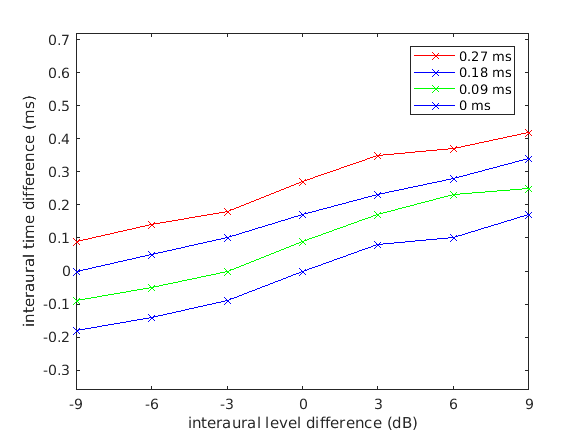
| 'fig17' | Return data from Fig. 17. The output data format is x-axis, 0ms, 0.09ms, 0.18ms, 0.27ms. The data is ITD vs. ILD. |
If no flag is given, the function will print the list of valid flags.
Examples:
Figure 11 with the "yost" condition can be displayed using
data_lindemann1986('fig11_yost','plot');
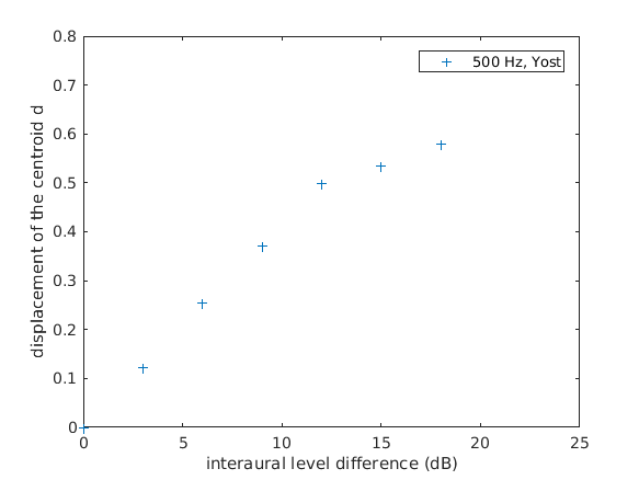
Figure 11 with the "sayers" condition can be displayed using
data_lindemann1986('fig11_sayers','plot');
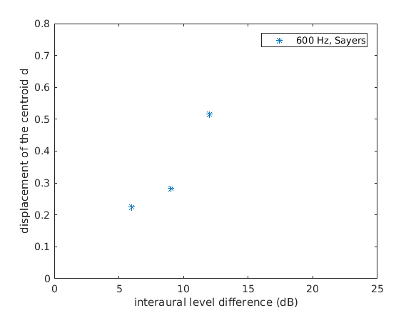
Figure 12 for a 400 Hz pure tone can be displayed using
data_lindemann1986('fig12_400','plot');
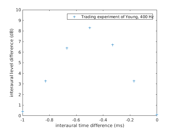
Figure 12 for a 600 Hz pure tone can be displayed using
data_lindemann1986('fig12_600','plot');
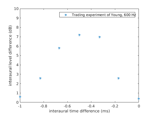
Figure 13 can be displayed by using
data_lindemann1986('fig13','plot');
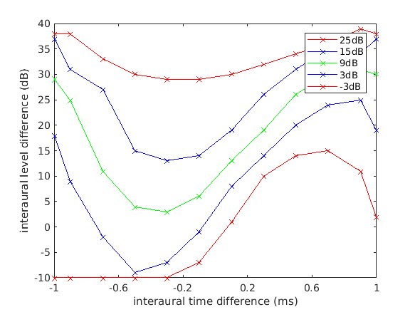
Figure 16 can be displayed using
data_lindemann1986('fig16','plot');
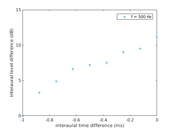
Figure 17 can be displayed using
data_lindemann1986('fig17','plot');
References:
W. Lindemann. Extension of a binaural cross-correlation model by contralateral inhibition. I. Simulation of lateralization for stationary signals. J. Acoust. Soc. Am., 80:1608--1622, 1986.


