Usage

plot_modspecgram(f,fs);
plot_modspecgram(f,fs,...);

Description

plot_modspecgram(f,fs) plot the modulation spectogram of the signal f sampled at a sampling frequency of fs Hz.

C=plot_modspecgram(f,fs, ... ) returns the image to be displayed as a matrix. Use this in conjunction with imwrite etc.

The function takes the following additional arguments

'win',g	Use the window g. See the help on gabwin for some possiblities. Default is to use a Gaussian window controlled by the 'thr' or 'wlen' parameters listed below.
'tfr',v	Set the ratio of frequency resolution to time resolution. A value \(v=1\) is the default. Setting \(v>1\) will give better frequency resolution at the expense of a worse time resolution. A value of \(0<v<1\) will do the opposite.
'wlen',s	Window length. Specifies the length of the window measured in samples. See help of PGAUSS on the exact details of the window length.
'image'	Use imagesc to display the spectrogram. This is the default.
'clim',clim	Use a colormap ranging from clim(1) to clim(2). These values are passed to imagesc. See the help on imagesc.
'dynrange',r	Use a colormap in the interval [chigh-r,chigh], where chigh is the highest value in the plot.
'fmax',fmax	Display fmax as the highest frequency.
'mfmax',mfmax	Display mfmax as the highest modulation frequency.
'xres',xres	Approximate number of pixels along x-axis / time.
'yres',yres	Approximate number of pixels along y-axis / frequency
'contour'	Do a contour plot to display the spectrogram.
'surf'	Do a surf plot to display the spectrogram.
'mesh'	Do a mesh plot to display the spectrogram.
'colorbar'	Display the colorbar. This is the default.
'no_colorbar'	Do not display the colorbar.
'interp'	Interpolate the image to get the desired x-resolution. Turn this off by using 'no_interp'

The parameters 'dynrange' and 'mfmax' may be speficied first on the argument line, in that order.

Examples:

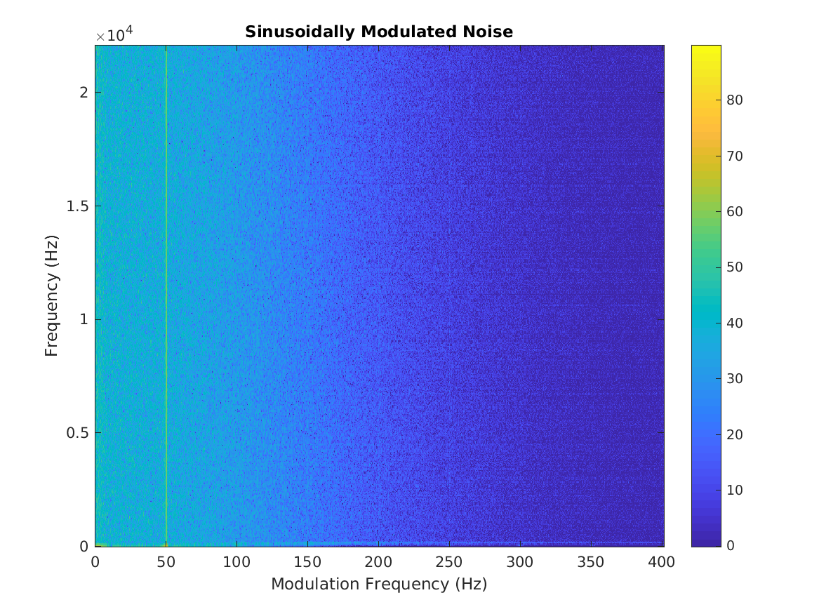
The first example shows a Modulation spectrogram of modulated wide band noise. The modulation frequency is 50 Hz and the signal is sampled at 44.1 kHz:

fm = 50;    % Modulation frequency
l = 2;      % Length of the signal in seconds
fs = 44100; % Sampling frequency
t = 0:1/fs:l;
n = length(t);
noise = 1-2*randn(1,n);
modnoise = noise.*(1+cos(2*pi*t*fm));
plot_modspecgram(modnoise,fs,90)
title('Sinusoidally Modulated Noise')

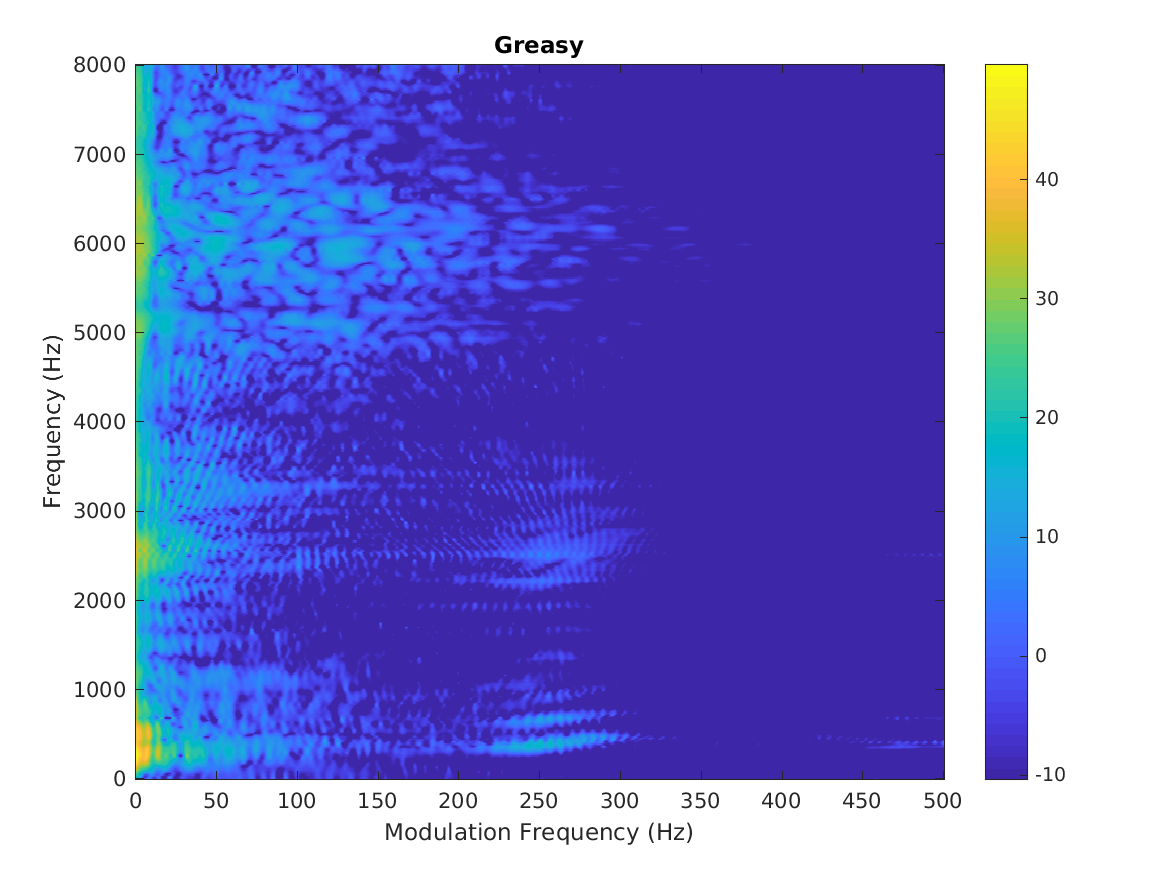
The second example shows a modulation spectrogram of a speech signal sampled at 16 kHz:

plot_modspecgram(greasy,16000,60,500)
title('Greasy')

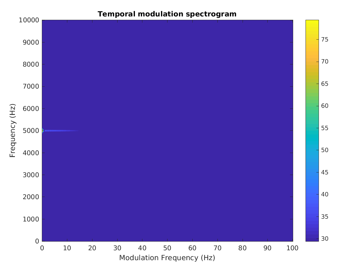
The third example shows a modulation spectrogram of a modulated sinusoid with a carrier frequency of 5 kHz. FIXME: What is the modulation frequency:

fm = 50;    % Modulation frequency
l = 2;      % Length of the signal in seconds
fs = 44100; % Sampling frequency
fc = 5000;  % Carrier frequency
t = 0:1/fs:l;
s = sin(2*pi*t*fc);
smod = s.*(1+0.5*cos(2*pi*t*fm));
plot_modspecgram(s,fs,50,2*fm,'fmax',2*fc)