THE AUDITORY MODELING TOOLBOX
Go to function
exp_felsheim2024
Reproduce figures from Felsheim and Dietz (2024)
Usage:
exp_felsheim2024(flag)
Description:
exp_felsheim2024(flag) reproduces the figures from Felsheim and Dietz (2024).
The following flags can be specified:
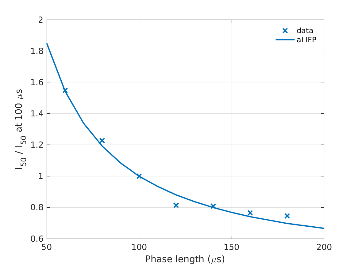
| 'fig5a' | The \(I_{50}\) (current amplitude at 50% firing probability) for biphasic pulses with different phase durations is shown, normalized on the \(I_{60}\) of the pulse with a 100-\(\mu s\) phase duration. The figure shows both the predictions by the aLIFP model and the data recorded by Shepherd and Javel (1999) from a single cat auditory nerve fiber. |
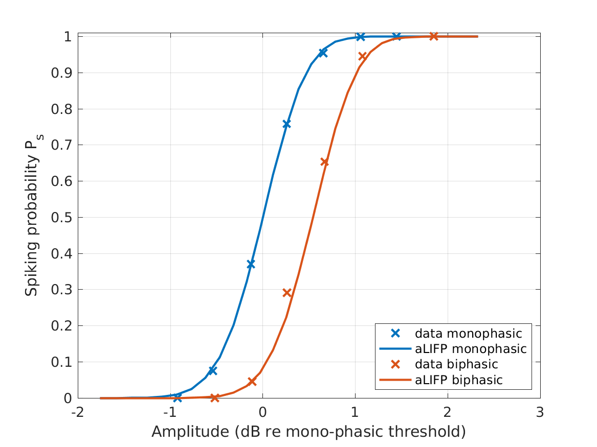
| 'fig5b' | The spike probability for different amplitdues for mono- and biphasic pulses with a phase duration 100 \(\mu s\) and 0 \(\mu s\) IPG are shown. The figure shows both the predictions by the aLIFP model and the data recorded by Shepherd and Javel (1999) from a single cat auditory nerve fiber. |
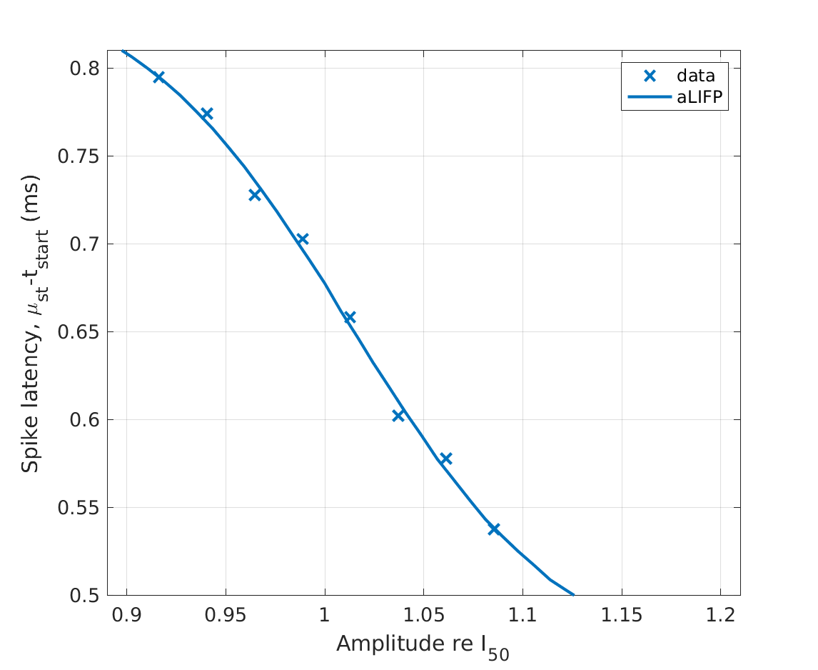
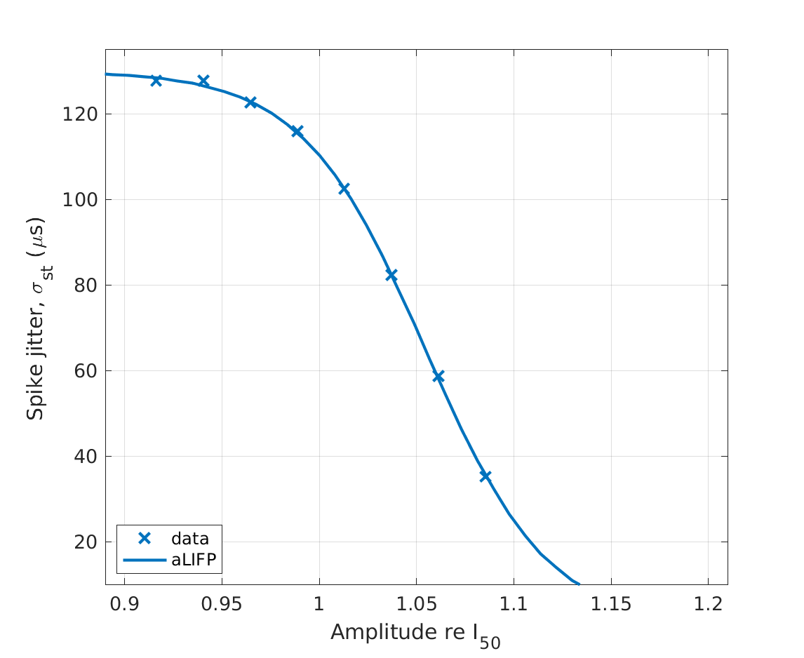
| 'fig5cd' | The spike latency (c) and the spike jitter (d) of monophasic pulses are shown. The data is shown togehter with the predictions of the aLIPF model and was collected by Miller et al. (1999), who used monophasic pulses with a duration of 40 \(\mu s\) and without IPG to stimulate a single cat auditory nerve fiber. |
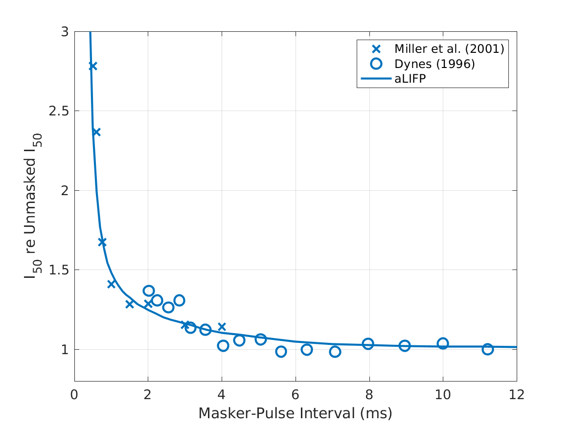
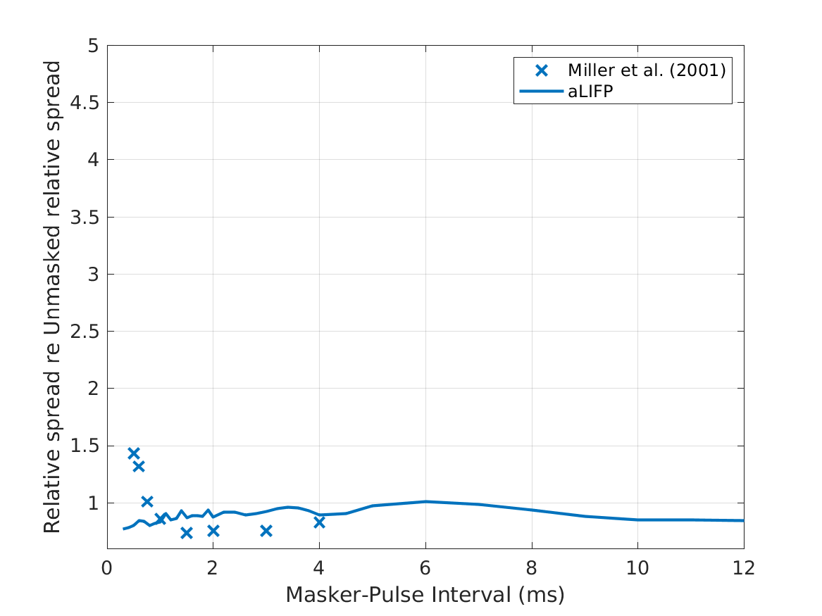
| 'fig6ab' | The mean I_50 (a) and relative spread (b) during the refractory period recorded with monophasic pulses with a length of 40 \(\mu s\) in 34 cat nerve fibers (Miller et al., 2001) and a length of 100 \(\mu s\) in 8 cat nerve fibers by (Dynes, 1996), together with the predictions made by the aLIFP. |
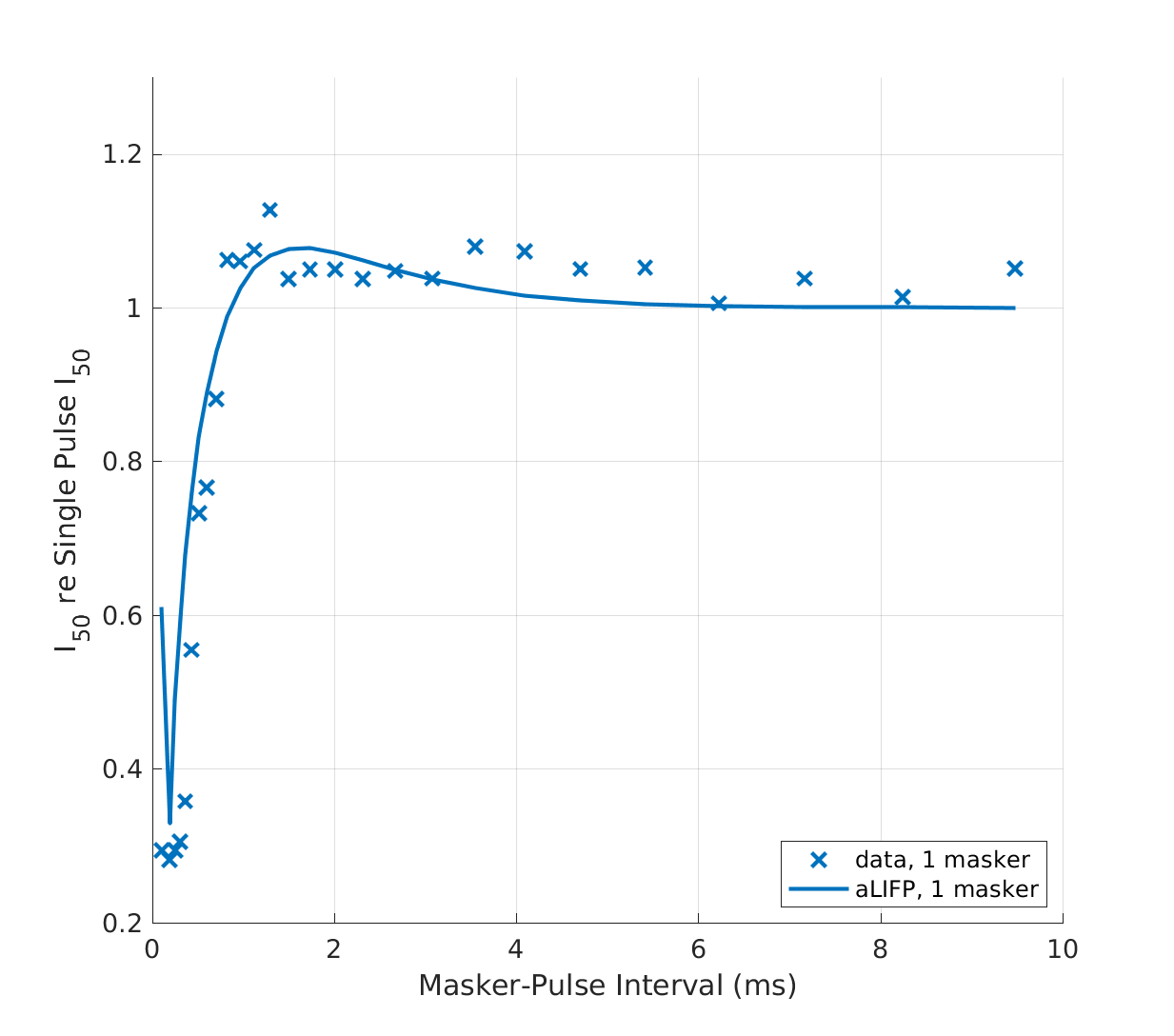
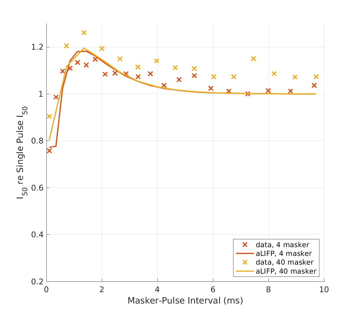
| 'fig6cd' | In (c), the data by Dynes (1996) for facilitation by a single sub-threshold pulse is shown, again, together with the predictions by both models and in (d), the same is shown for four and 40 sub-threshold masker. Dynes (1996) used monophasic pulses with a duration of 100 \(\mu s\). |
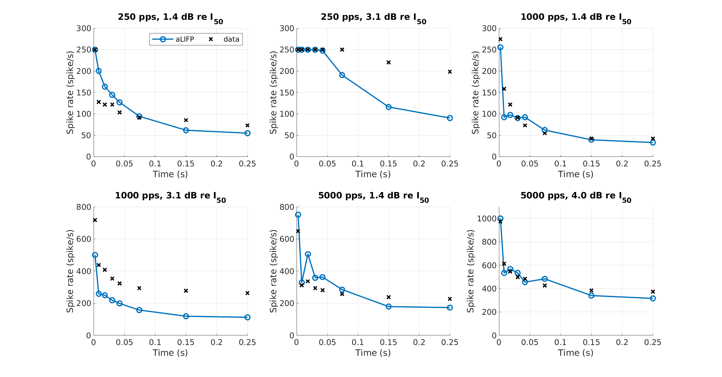
| 'fig6e' | The spike rate adaptation for different pulse rates and amplitudes, as measured by Zhang et al. (2007). Our model was fitted at two amplitudes for each of the pulse rates 250 pps, 1000 pps, and 5000 pps. The low amplitude was always 1.4 dB re \(I_{50}\). For 250 pps and 1000 pps the high amplitude was 3.1 dB re \(I_{50}\) and for 5000 pps the high amplitude was 4.0 dB re \(I_{50}\). Note the slightly higher second amplitude for 5000 pps, which was used according to the data. . |
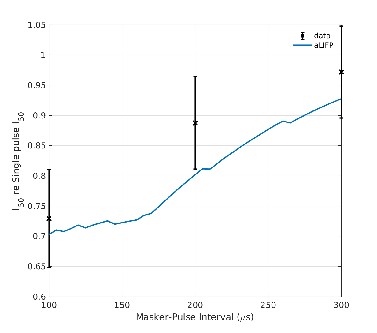
| 'fig7' | The decrease in threshold due to facilitation is measured by Cartee et al. (2000) by dividing the \(I_{50}\) of two pseudo-monophasic pulses by the \(I_{50}\) of a single of these pulses. The data was collected by Cartee et al. (2000) using 38 cat nerve fibers and is compared to predictions of the aLIFP model. |
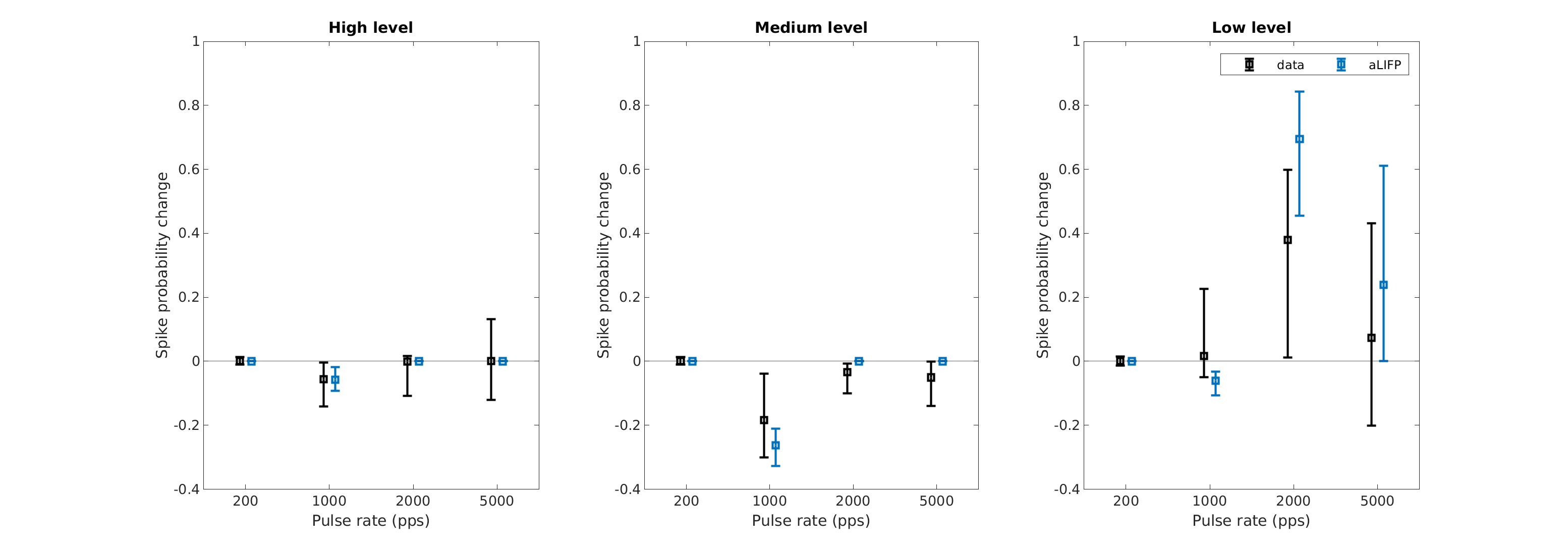
| 'fig8' | Facilitation and accommodation as calculated from spike trains by Heffer et al. (2010). Negative values indicate accommodation, while positive ones denote facilitation. The predictions from the aLIFP model fit the data nicely, except for 2000 pps at low levels, where the aLIFP model overestimates the facilitation. |
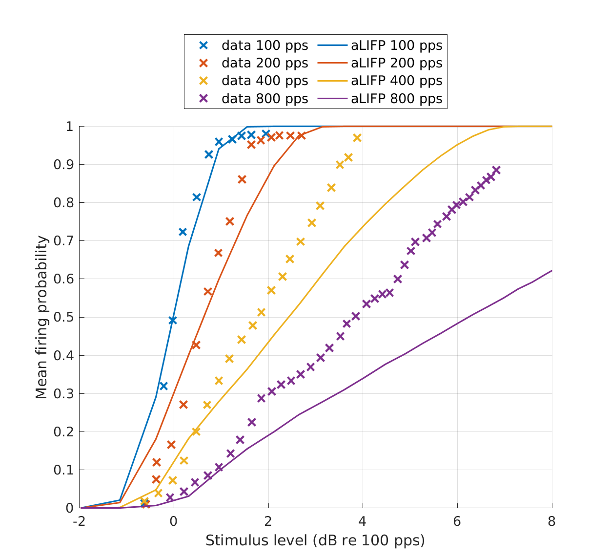
| 'fig9' | Mean firing probability over level for four 100 \(\mu s\) pulse trains with different pulse rates. The x-axes give the amplitude in dB re \(I_{50}\) at 100 pps. The data were collected on a single cat nerve fiber by Javel (1990) and simulated using the aLIFP model. |
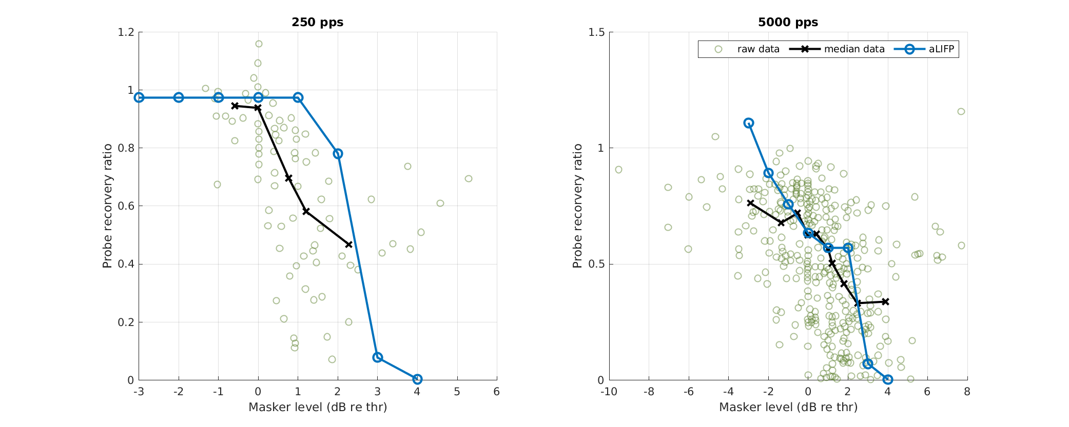
| 'fig10' | Data collected by Miller et al. (2011), who measured the impact of a low amplitude stimulus on a subsequent probe in 48 cat nerve fibers. The amplitudes were placed around the spike threshold for the masker, defined as the level where firing just started. |
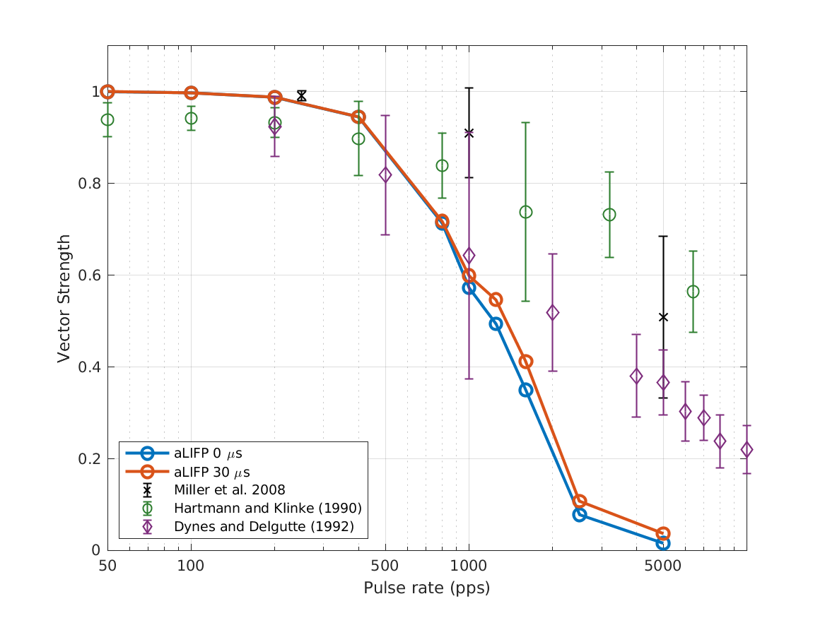
| 'fig11' | The vector strength from Miller et al. (2008), Hartmann and Klinke (1990) and Dynes and Delgutte (1992) for different pulse rates measured in cats. As the were made both for duration of the IPG was not clear, the predictions an IPG of 0 \(\mu s\) and 30 \(\mu s\). The predictions of the aLIFP model are not affected by the IPG and it fits the data for both pulse shapes up to 1600 pps. |
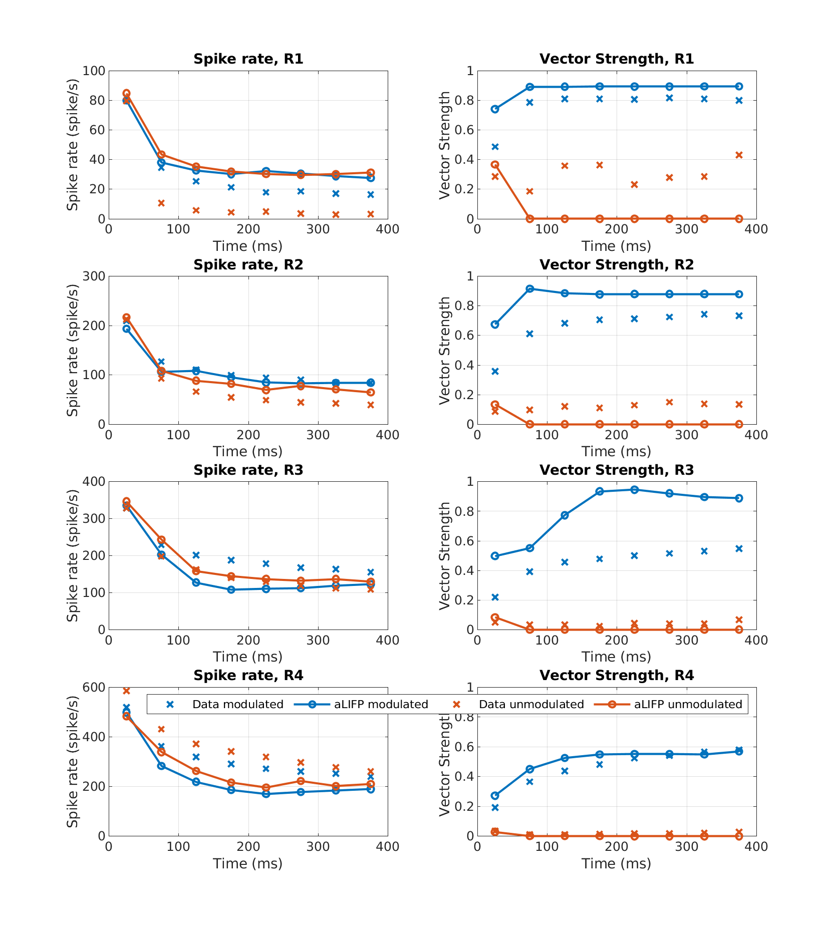
| 'fig12' | The spike rate and the vector strength of 100 Hz sinusoidally amplitude modulated and unmodulated pulse trains with a rate of 5000 pps were calculated. The predictions the aLIFP model were compared to data of 72 cat nerve fibers from Hu et al. (2010). |
| 'figA1' | The vector strength obtained from the predictions of the aLIFP model for different IPG durations and two amplitudes: 1 dB and 2 dB relative to single pulse \(I_{50}\). The left plot shows the predictions for a 2500 pps stimulus and the right one for a 5000 pps stimulus, both with a duration of 0.3 s. For the 5000 pps stimulus the calculations could only reasonably be performed up to 50 \(\mu s\) IPG, because for higher IPG values the gap between the pulses would have been shorter than the IPG. |
| 'redo' | Force recalculation of the data. Cached data are shown per default. |
Examples:
To display Fig. 5a use :
exp_felsheim2024('fig5a');
|
|
To display Fig. 5b use :
exp_felsheim2024('fig5b');
|
|
To display Fig. 5cd use :
exp_felsheim2024('fig5cd');
|
|
|
To display Fig. 6ab use :
exp_felsheim2024('fig6ab');
|
|
|
To display Fig. 6cd use :
exp_felsheim2024('fig6cd');
|
|
|
To display Fig. 6e use :
exp_felsheim2024('fig6e');
|
|
To display Fig. 7 use :
exp_felsheim2024('fig7');
|
|
To display Fig. 8 use :
exp_felsheim2024('fig8');
|
|
To display Fig. 9 use :
exp_felsheim2024('fig9');
|
|
To display Fig. 10 use :
exp_felsheim2024('fig10');
|
|
To display Fig. 11 use :
exp_felsheim2024('fig11');
|
|
To display Fig. 12 use :
exp_felsheim2024('fig12');
|
|
References:
R. C. Felsheim and M. Dietz. An adaptive leaky integrate and firing probability model of an electrically stimulated auditory nerve fiber. Trends in Heaaring, 2024. submitted.


Build with Bootstrap